2023-08-31__STA_conntest¶

So, hi. copying from prev nb:

So, for all 10 Ns;
For 10 diff seeds; for both exc, inh, and unconn;
we conntest (maximum) 100 input spike trains.
(Each test is comprised of calculating 101 STAs: one real and the rest with shuffled ISIs).

include("lib/Nto1.jl")

using Revise … ✔
using Units, Nto1AdEx, ConnectionTests, ConnTestEval … ✔
using StatsBase … ✔

duration = 10minutes
N = 6500

@time sim = Nto1AdEx.sim(N, duration);

  3.184070 seconds (2.14 M allocations: 1.027 GiB, 2.32% gc time, 42.19% compilation time)

(So even with native code caching in Julia 1.9, we still have 30% of time compilation here).

We decided we’d pick the 100 highest firing (exc and inh).
And then generate some unconnecteds too..
What’s their firing rate? Maybe sample from the real ones :) hehe, sure.

Gen unconnected trains¶

exc_inputs = highest_firing(excitatory_inputs(sim))[1:100]
inh_inputs = highest_firing(inhibitory_inputs(sim))[1:100]
both = [exc_inputs..., inh_inputs...]
fr = spikerate.(both)
showsome(fr / Hz)

200-element Vector{Float64}:
   1: 97.5
   2: 58.9
   ⋮
  31: 21.5
   ⋮
 146: 12.5
   ⋮
 199: 8.87
 200: 8.86

Random.seed!(1)
unconn_frs = sample(fr, 100)
showsome(unconn_frs)

100-element Vector{Float64}:
   1: 25.9
   2: 17.1
   ⋮
  19: 17.7
   ⋮
  72: 11
   ⋮
  99: 10.4
 100: 8.92

Seed may not be same as seed in sim: otherwise our ‘unconnected’ trains generated might be same as real ones used in (generated in) sim.

Random.seed!(9)
unconn_trains = [poisson_SpikeTrain(r, duration) for r in unconn_frs];

Conntest¶

ConnectionTests.set_STA_length(200);  # = 20 ms

test(train) = test_conn(STAHeight(), sim.V, train.times)

@time test(exc_inputs[1])

  1.280038 seconds (1.58 M allocations: 240.340 MiB, 4.21% gc time, 58.25% compilation time)

0.94

(That value is the ‘connectedness measure’ I defined. Here simply 1 – p-value)

Plottin some unconnected STAs.

include("lib\\plot.jl")

import PythonCall … ✔ (2.3 s)
import PythonPlot … ✔ (6 s)
using Sciplotlib … ✔ (0.6 s)
using PhDPlots … ✔

_plotSTA(train, winlength = 1000; kw...) = plotSTA(calc_STA(sim.V, train.times, Nto1AdEx.Δt, winlength); kw...);
fig, axs = plt.subplots(ncols=2, figsize=(pw, 0.3pw), sharey=true)
_plotSTA(exc_inputs[1], ax=axs[0])
_plotSTA(unconn_trains[1], ax=axs[0], c="gray")
_plotSTA(unconn_trains[2], ax=axs[1], c="gray")
_plotSTA(unconn_trains[3], ax=axs[1], c="black");

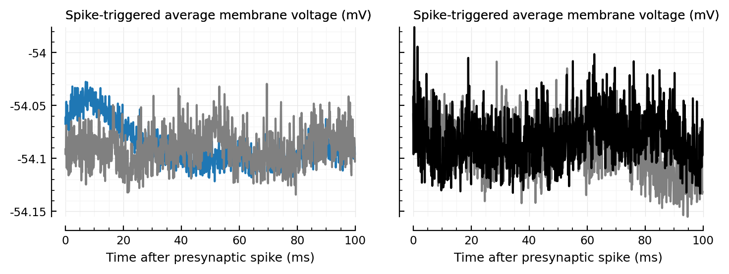
../_images/2023-08-31__STA_conntest_17_0.png

@time test.(unconn_trains[[1,2,3]])

  0.653168 seconds (87.31 k allocations: 84.142 MiB, 10.37% compilation time)

3-element Vector{Float64}:
 -0.01
 -0.02
 -0.94

include("lib/df.jl")

using DataFrames … ✔ (0.9 s)

using ProgressMeter

rows = []

@time for (conntype, trains) in [
        (:exc, exc_inputs),
        (:inh, inh_inputs),
        (:unc, unconn_trains)
    ]
    descr = string(conntype)
    @showprogress descr for train in trains
        t = test(train)
        fr = spikerate(train)
        push!(rows, (; conntype, fr, t))
    end
end;

exc 100%|████████████████████████████████████████████████| Time: 0:00:23mm39mm
inh 100%|████████████████████████████████████████████████| Time: 0:00:16
unc 100%|████████████████████████████████████████████████| Time: 0:00:20
 60.244557 seconds (1.78 M allocations: 7.140 GiB, 1.40% gc time, 2.27% compilation time)

showsome(rows)

300-element Vector{Any}:
   1: (conntype = :exc, fr = 97.5, t = 0.94)
   2: (conntype = :exc, fr = 58.9, t = 0.95)
   ⋮
  34: (conntype = :exc, fr = 21.1, t = 0.86)
   ⋮
 167: (conntype = :inh, fr = 10.4, t = 0.93)
   ⋮
 299: (conntype = :unc, fr = 10.3, t = 0.6)
 300: (conntype = :unc, fr = 8.81, t = 0.39)

df = DataFrame(rows)
rename!(df, :fr => "Spikerate (Hz)")

300×3 DataFrame

290 rows omitted

Row	conntype	Spikerate (Hz)	t
	Symbol	Float64	Float64
1	exc	97.5	0.94
2	exc	58.9	0.95
3	exc	40.7	0.99
4	exc	34.4	0.54
5	exc	31.5	0.87
&vellip;	&vellip;	&vellip;	&vellip;
296	unc	9.21	0.94
297	unc	16.4	0.29
298	unc	8.98	-0.96
299	unc	10.3	0.6
300	unc	8.81	0.39

Eval¶

sweep = ConnTestEval.sweep_threshold(df);

showsome(sweep.threshold)

96-element Vector{Float64}:
  1: 0.99
  2: 0.98
  ⋮
 39: 0.6
  ⋮
 79: 0.19
  ⋮
 95: 0.01
 96: 0

23/100

0.23

predtable = at_FPR(sweep, 5/100)
print_confusion_matrix(predtable)

              Predicted
           exc   inh   unc
      exc    6     2    92
Real  inh    0     6    94
      unc    4     2    94

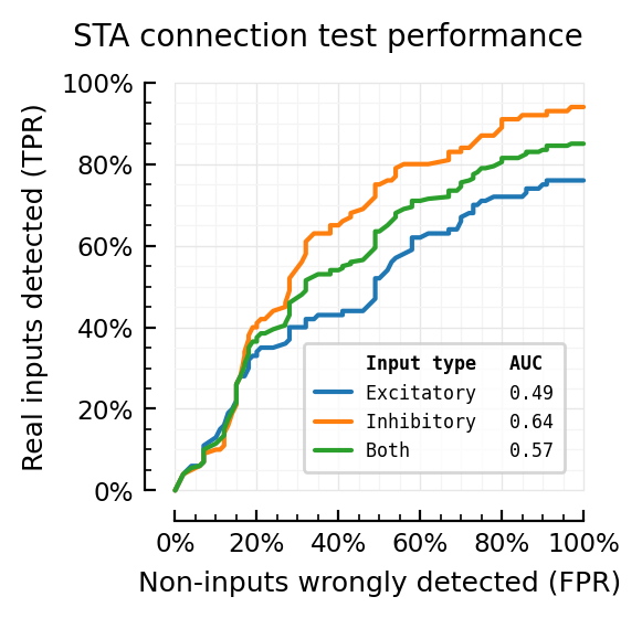
AUCs = calc_AUROCs(sweep)
AUCs = (; (k=>round(AUCs[k], digits=2) for k in keys(AUCs))...)

(AUC = 0.57, AUCₑ = 0.49, AUCᵢ = 0.64)

Damn! This was when not ceiling spikes:

              Predicted
           exc   inh   unc
      exc   23     3    74
Real  inh    0    40    60
      unc    4     2    94

(AUC = 0.77, AUCₑ = 0.68, AUCᵢ = 0.86)

fig, ax = plt.subplots()
# ax.axvline(0.05, color="gray", lw=1)
plot(sweep.FPR, sweep.TPRₑ; ax, label="Excitatory   $(AUCs.AUCₑ)")
plot(sweep.FPR, sweep.TPRᵢ; ax, label="Inhibitory   $(AUCs.AUCᵢ)")
plot(sweep.FPR, sweep.TPR; ax,  label="Both         $(AUCs.AUC)")
set(ax, aspect="equal", xlabel="Non-inputs wrongly detected (FPR)", ylabel="Real inputs detected (TPR)",
    xtype=:fraction, ytype=:fraction, title=("STA connection test performance", :pad=>12, :loc=>"right"))
font = Dict("family"=>"monospace", "size"=>6)
legend(ax, borderaxespad=1,     title="Input type   AUC ", loc="lower right",
        alignment="right", markerfirst=true, prop=font);
# Using the same `font` dict for `title_fontproperties` does not apply the size (bug ig)
# (bug in this PR? https://github.com/matplotlib/matplotlib/pull/19304)
# Hm, it works in straight Python[*]. Interesting.
ax.legend_.get_title().set(family="monospace", size=6, weight="bold");

../_images/2023-08-31__STA_conntest_31_0.png

[*]: http://localhost:8888/notebooks/2023-09-05__mpl_legend_title_props_bugreport.ipynb

(below not updated after adding ceil_spikes=true)

neighbours_of_5pct_line = sweep[5:6]
neighbours_of_5pct_line.threshold

2-element Vector{Float64}:
 0.95
 0.94

neighbours_of_5pct_line.FPR

2-element Vector{Float64}:
 0.03
 0.06

Sudden jump in TPRs right around 5%.
Coincidence I think, cause there is no threshold programmed in STAHeight ConnectionTest.

Actually no, jump is after 5% / at 6%:

x = sweep[5:11]
DataFrame(; x.threshold, x.FPR, x.TPR)

7×3 DataFrame

Row	threshold	FPR	TPR
	Float64	Float64	Float64
1	0.95	0.03	0.28
2	0.94	0.06	0.315
3	0.93	0.06	0.335
4	0.92	0.06	0.4
5	0.91	0.06	0.44
6	0.9	0.06	0.465
7	0.89	0.07	0.48

So we increase the threshold from 0.94 to 0.90, and find more TPs, without incurring any additional FPs.

Voltage-to-Wiring Sim

2023-08-31__STA_conntest

Contents

2023-08-31__STA_conntest¶

Gen unconnected trains¶

Conntest¶

Eval¶