2023-01-19 • Fit a line
Contents
2023-01-19 • Fit a line
We’re working off 2022-10-24 • N-to-1 with lognormal inputs.
But trying a new detection method.
(Linear regression of voltage against time-post-spike)
Note that, unlike in earlier sims, there is no transmission delay added in the latest sim.
Setup
I’ll put the work from previous notebook in a script (not package, this time)
(Thanks to ‘jupytext’ extension, that script’ll also be a notebook)
include("2023-01-19__[input].jl");
using Revise: 2.418806 seconds (603.38 k allocations: 36.618 MiB, 4.00% gc time, 1.02% compilation time)
WARNING: using MyToolbox.@withfb in module Main conflicts with an existing identifier.
using MyToolbox: 5.079011 seconds (1.63 M allocations: 103.773 MiB, 2.95% gc time, 0.44% compilation time)
using SpikeWorks: 2.238519 seconds (1.28 M allocations: 78.599 MiB, 5.98% gc time)
using Sciplotlib: 26.325986 seconds (7.10 M allocations: 455.083 MiB, 1.64% gc time, 2.21% compilation time: 100% of which was recompilation)
using VoltoMapSim: 14.394408 seconds (4.98 M allocations: 328.898 MiB, 3.82% gc time)
Loading cached output from `/root/.phdcache/runsim/2023-01-19__[input]__N=5.jld2` … done (17.3 s)
Loading cached output from `/root/.phdcache/runsim/2023-01-19__[input]__N=20.jld2` … done (0.3 s)
Loading cached output from `/root/.phdcache/runsim/2023-01-19__[input]__N=100.jld2` … done (0.3 s)
Loading cached output from `/root/.phdcache/runsim/2023-01-19__[input]__N=400.jld2` … done (0.3 s)
Loading cached output from `/root/.phdcache/runsim/2023-01-19__[input]__N=1600.jld2` … done (2.6 s)
Loading cached output from `/root/.phdcache/runsim/2023-01-19__[input]__N=6500.jld2` … done (4.5 s)
(I disabled STA calculating/caching/loading in there: we’re gon work on individual windows).
Start
We’ll tackle the most difficult case.
i = 6
6
N = Ns[i]
6500
sim = sims[i]
Simulation{Nto1System{NeuronModel{NamedTuple{(:v, :u, :gₑ, :gᵢ), NTuple{4, Float64}}, typeof(f!), typeof(has_spiked), typeof(on_self_spike!)}, var"#on_spike_arrival!#9"{Float64, Float64, var"#neuron_type#8"{Int64}}}, CVec{(:v, :u, :gₑ, :gᵢ)}}
Summary: completed. 5.3 spikes/s
Properties:
       system: Nto1System, x₀: (v = -0.05, u = 0, gₑ = 0, gᵢ = 0), input feed: all 19426057 spikes processed
           Δt: 0.0001
     duration: 600
  stepcounter: 6000000 (complete)
        state: t = 600 seconds, neuron = vars: (v: -0.0374, u: -2.95E-11, gₑ: 3.59E-09, gᵢ: 2.45E-09), Dₜvars: (v: 0.994, u: -4.64E-10, gₑ: -5.2E-07, gᵢ: -3.55E-07)
          rec: v: [-0.0501, -0.0501, -0.0502, -0.0503, -0.0504, -0.0504, -0.0505, -0.0506, -0.0506, -0.0507  …  -0.0383, -0.0382, -0.0381, -0.038, -0.0379, -0.0378, -0.0377, -0.0376, -0.0375, -0.0374], spiketimes: [0.116, 0.264, 0.504, 0.68, 0.881, 1.08, 1.25, 1.46, 1.66, 1.84  …  598, 598, 598, 599, 599, 599, 599, 600, 600, 600]
spikerate(sim) / Hz # ..of the single output neuron
5.29
inp = inps[i];
So we could fit an STA. then there’s one y per x; a 100 xs (for 10 ms post ‘arrival’).
Or we could do individual windows. Let’s do that. (How many datapoints then?
50 Hz input for 10minutes:
_numspikes = 50Hz*10minutes
3E+04
So 30_000 windows. And 30_000 y’s per x. (per t, actually)
Let’s find highest spiking exc neuron
actual_spike_rates = spikerate_.(inp.inputs);
for f in [minimum, median, mean, maximum]
    println(lpad(f, 8), ": ", f(actual_spike_rates), " Hz")
end
 minimum: 0.338 Hz
  median: 3.96 Hz
    mean: 4.98 Hz
 maximum: 63.5 Hz
Nₑ = inp.Nₑ
5200
_, ni = findmax(actual_spike_rates)
(63.5, 3743)
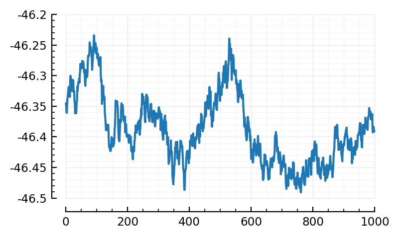
calcSTA(ni) = calcSTA(sim, spiketimes(inp.inputs[ni]))

plot(calcSTA(ni) / mV);
But we’re not fitting STAs, we’re fitting indiv windows. So.
(Wow, this one (3743, on WSL) is weird).
Windows
function windows(v, times, Δt, winsize)
    # Assuming that times occur in [0, T)
    win_starts = floor.(Int, times / Δt) .+ 1
    wins = Vector{Vector{eltype(v)}}()
    for a in win_starts
        b = a + winsize - 1
        if b ≤ lastindex(v)
            push!(wins, v[a:b])
        end
    end
    return wins
end

windows(spiketimes) = windows(
    vrec(sim),
    spiketimes,
    Δt,
    winsize,
)

windows(i::Int) = windows(spiketimes(inp.inputs[i]));
# check for type inferrability
# st = spiketimes(inp.inputs[1])
# @code_warntype windows(vrec(sim), st, Δt, winsize)
# ok ✔
@time wins = windows(ni);
println()
print(Base.summary(wins))
  1.248030 seconds (97.44 k allocations: 300.789 MiB, 20.77% gc time)

38091-element Vector{Vector{Float64}}
Now to make the data matrix
Data matrix
We’ll fit slope and intercept. So each datapoint, each row of X, is [1, t]
function build_Xy(windows, timepoints = 1:100)
    T = eltype(eltype(windows))
    N = length(windows) * length(timepoints)
    X = Matrix{T}(undef, N, 2)
    y = Vector{T}(undef, N)
    i = 1
    for win in windows
        for (tᵢ, yᵢ) in zip(timepoints, win[timepoints])
            X[i,:] .= [1, tᵢ]
            y[i] = yᵢ
            i += 1
        end
    end
    @assert i == N + 1
    return (X, y)
end


@time X, y = build_Xy(wins);
2.270752 seconds (4.09 M allocations: 426.801 MiB, 6.93% gc time)
# check for type inferrability
# @code_warntype build_Xy(wins, 1:100)
# ok ✔
size(X)
(3809100, 2)
size(y)
(3809100,)
Some example data:
_r = 95:105

[X[_r, :] y[_r] / mV]
11×3 Matrix{Float64}:
 1   95  -46.5
 1   96  -46.5
 1   97  -46.5
 1   98  -46.5
 1   99  -46.5
 1  100  -46.5
 1    1  -45.2
 1    2  -45.2
 1    3  -45.2
 1    4  -45.2
 1    5  -45.2
So for our model y = ax + b (w/ β = [b, a])
x is in units of ‘timestep’
So a will be too: mV/timestep
Solve
Linear regression assuming Gaussian noise → MSE, ‘OLS’, normal equations
?\ → “\(X,y) for rectangular X:
minimum-norm least squares solution computed by
a pivoted QR factorization of X
and a rank estimate of X based on the R factor”
@time β̂ = X \ y
0.311424 seconds (31 allocations: 87.250 MiB)
2-element Vector{Float64}:
 -0.0463
  9.59E-07
(First run time i.e. including compilation: 4 seconds)
intercept = β̂[1] / mV
-46.3
Ok check
For the slope,
slope = β̂[2] / mV
0.000959
That’s per timestep.
Per second:
slope / Δt
9.59
Plot some windows
ts = @view X[:,2]
sel = 1:10000

plot(ts[sel]*Δt/ms, y[sel]/mV, ".", alpha=0.1);
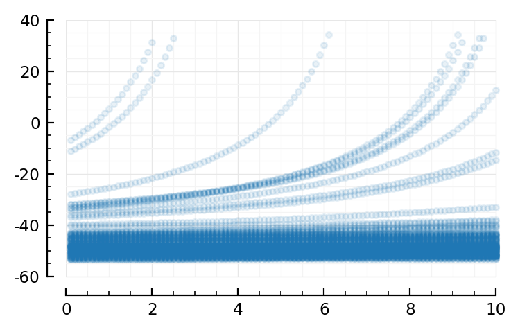
It’s the spikes we see there.
(and the unrealistically slow quadratic ramp-ups of Izhikevich)
so let’s zoom in
Ny = length(y)
3809100
3M datapoints (one connection, 10 minutes recording)
sel = 1:100_000

plot(
    ts[sel]*Δt/ms,
    y[sel]/mV,
    ".";
    alpha = 0.01,
    ylim = [-50, -40],  # mV
    clip_on = true,
);
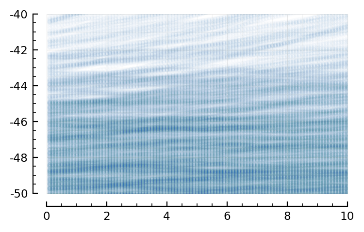
(Not very informative)
Use as conntest
(We could look at uncertainty / goodness of fit but not now)
First, let’s see what fitted slope is for an inh input; and a shuffled one.
inh_neurons = Nₑ+1:N
5201:6500
niᵢ = Nₑ + argmax(actual_spike_rates[inh_neurons])
5798
actual_spike_rates[niᵢ] / Hz
43.9
"""
Fit straight line to first 100 ms of
windows cut out of output neuron's voltage signal,
aligned to given times `z`
(or spiketimes of input neuron w/ index `z`).
"""
fitwins(z) = begin
    wins = windows(z)
    X, y = build_Xy(wins)
    β̂ = vec(X \ y)
    ŷ = X * β̂
    ε̂ = y .- ŷ
    return (;
        X, y, β̂,
        intercept   = β̂[1] / mV,       # in mV
        slope       = β̂[2] / mV / Δt,  # in mV/second
        predictions = ŷ,
        residuals   = ε̂,
    )
end;
# check for type inferrability
# @code_warntype fitwins(niᵢ)
# ok ✔
@time fitwins(niᵢ).slope
1.573785 seconds (2.69 M allocations: 589.847 MiB, 22.97% gc time)
-26
(First run time: 2.7 seconds)
niₑ = ni
3743
@time fitwins(niₑ).slope
2.091091 seconds (3.89 M allocations: 852.352 MiB, 12.40% gc time)
9.59
spiketimes(i::Int) = spiketimes(inp.inputs[i])

stₑ = spiketimes(niₑ)

@time fitwins(shuffle_ISIs(stₑ)).slope
2.472024 seconds (4.60 M allocations: 902.115 MiB, 6.14% gc time)
8.06
Okido
Now, to use as conntest.
Null hypothesis is that slope = 0
Refresher at https://gregorygundersen.com/blog/2021/09/09/ols-hypothesis-testing/
Hypothesis testing
If the slope actually were 0
(i.e. \(b_p = b_1 = 0\) in the post),
(and if noise were gaussian, which it’s not given the assymetric spiking)
then we expect the slope (“\(β̂_1\)”), to be distributed as:
where \(Q\) is the inverse of the Gram matrix \(X^T X\):
(\(Q\) ‘is related to’ the covariance matrix, and is called the cofactor matrix.
https://en.wikipedia.org/wiki/Ordinary_least_squares#Estimation)
..and with \(σ\) the (unkown) standard-deviation of our supposedly-Gaussian-distributed noise \(ε\) in our model
i.e.
(‘\(Q_{[2,2]}\)’ is the second diagonal element of \(Q\). The indices are off-by-one as the intercept is conventionally \(β_0\) instead of \(_1\)).
Estimate noise on model
fitt = fitwins(niₑ);
n = length(fitt.y)
p = 2  # Num params
dof = n - p
3809098
ε̂ = fitt.residuals;
OLS estimate of variance σ² of Gaussian noise ε:
s² = ε̂' * ε̂ / dof
7.59E-05
MLE estimate:
σ̂² = ε̂' * ε̂ / n
7.59E-05
(ofc virtually same cause ridic amount of datapoints)
So estimate for stddev of noise on our line, in mV:
√s² / mV
8.71
Seems about right.
Gram matrix
X = fitt.X
G = X' * X  # not calling it N, that's used already
2×2 Matrix{Float64}:
 3.81E+06  1.92E+08
 1.92E+08  1.29E+10
Q = inv(G)
2×2 Matrix{Float64}:
  1.07E-06  -1.59E-08
 -1.59E-08   3.15E-10
So, estimated stddev of our slope distribution.
σ̂β₂ = √(s² * Q[2,2])
1.55E-07
σ̂β₂ / mV
0.000155
Aka standard error or ‘se(\(\hat{β}_2\))’
t-statistic
Slope in mV:
fitt.slope
9.59
In original units of the (X,y) fit, i.e. volt/timestep:
β̂₂ = fitt.β̂[2]
9.59E-07
t = β̂₂ / σ̂β₂
6.21
That value follows the Student’s t-distribution with n-p degrees of freedom,
which, at our
dof
3809098
is same as Normally distributed.
using Distributions
𝒩 = Normal()
Normal{Float64}(μ=0, σ=1)
Null-hypothesis is that slope == 0.
So alternative is that it can be both larger and smaller.
Critical values:
α = 0.05
0.05
quantile(𝒩, α/2)
-1.96
cquantile(𝒩, α/2)
1.96
So yes our slope is significant.
By how much, i.e. what’s p-value
I.e. probability of t being at least this large, under H₀.
pval = cdf(𝒩, -t) + ccdf(𝒩, t)
5.45E-10
i.e. p < 0.05
This happens by chance once in
1/pval
1.84E+09
1_8400_000_000 universes.
Now to package this up in a function
Summary
function htest(fit)
    (; X, y, β̂) = fit
    n = length(y)
    p = 2  # Num params
    dof = n - p
    ε̂ = fit.residuals
    s² = ε̂' * ε̂ / dof
    Q = inv(X' * X)
    σ̂β₂ = √(s² * Q[2,2])
    t = β̂[2] / σ̂β₂
    𝒩 = Normal(0, 1)
    pval = cdf(𝒩, -abs(t)) + ccdf(𝒩, abs(t))
    noise_mV = √s² / mV
    return (; t, pval, noise_mV)
end;
htest(fitt)
(t = 6.21, pval = 5.45E-10, noise_mV = 8.71)
@time htest(fitt);
0.046876 seconds (6 allocations: 1.422 KiB)
That’s fast :)
function conntest(z; α = 0.05)
    fit = fitwins(z)
    test = htest(fit)
    if test.pval < α
        predtype = (fit.slope > 0 ? :exc : :inh)
    else
        predtype = :unconn
    end
    return (;
        fit.slope,
        test.pval,
        predtype,
    )
end;
conntest(niₑ)
(slope = 9.59, pval = 5.45E-10, predtype = :exc)
conntest(niᵢ)
(slope = -26, pval = 2.57E-45, predtype = :inh)
Let’s try on shuffled spiketrains
shuffled(ni) = shuffle_ISIs(spiketimes(ni));
conntest(shuffled(niₑ))
(slope = 9.39, pval = 6.16E-10, predtype = :exc)
conntest(shuffled(niₑ))
(slope = -9.01, pval = 2.53E-09, predtype = :inh)
conntest(shuffled(niᵢ))
(slope = 16.2, pval = 1.22E-18, predtype = :exc)
That’s not great.
(In previous iteration of this notebook, with a different sim, all three of these were :unconn)
Eval
DataFrame(conntest(shuffled(niₑ)) for _ in 1:10)
| Row | slope | pval | predtype |
|---|---|---|---|
| Float64 | Float64 | Symbol | |
| 1 | -2.55 | 0.0967 | unconn |
| 2 | 1.99 | 0.188 | unconn |
| 3 | 4.37 | 0.00358 | exc |
| 4 | 6.25 | 3.39E-05 | exc |
| 5 | 2.97 | 0.0498 | exc |
| 6 | -2.87 | 0.0568 | unconn |
| 7 | 2.43 | 0.109 | unconn |
| 8 | -3.28 | 0.0308 | inh |
| 9 | 6.62 | 1.36E-05 | exc |
| 10 | 4.8 | 0.00166 | exc |
Ok this is similar as in prev instantiation of this notebook / prev sim.
(The three unconns above were thus lucky).
Proper eval
I didn’t sim a 100 unconnected spikers, as before.
So we can’t use that for an FPR estimate.
But we can shuffle some real spiketrains to get sth similar.
Let’s draw from all, so there’s a mix of spikerates.
ids = sample(1:N, 100, replace=true)
unconnected_trains = shuffle_ISIs.(spiketimes.(ids));
Our perftable expects a dataframe with :predtype and :conntype columns
inh_neurons
5201:6500
real_spiketrains = spiketimes.(1:N);
all_spiketrains = [real_spiketrains; unconnected_trains];
conntype(i) =
    if i < Nₑ
        conntype = :exc
    elseif i ≤ N
        conntype = :inh
    else
        conntype = :unconn
    end

makerow(i; α=0.001) = begin
    spikes = all_spiketrains[i]
    test = conntest(spikes; α)
    (; conntype = conntype(i), test...)
end;
@time makerow(1)
0.075884 seconds (312.28 k allocations: 68.547 MiB)
(conntype = :exc, slope = 17.9, pval = 0.000771, predtype = :exc)
@time makerow(6600)
0.077716 seconds (236.50 k allocations: 51.938 MiB)
(conntype = :unconn, slope = 11.6, pval = 0.0702, predtype = :unconn)
conntest_all() = @showprogress map(makerow, eachindex(all_spiketrains))

rows = cached(conntest_all, [], key="2023-01-19__Fit-a-line");
Progress: 100%|█████████████████████████████████████████| Time: 0:10:16
Saving output at `/root/.phdcache/conntest_all/2023-01-19__Fit-a-line.jld2` … done (5.0 s)
df = DataFrame(rows)
df |> disp(20)
| Row | conntype | slope | pval | predtype |
|---|---|---|---|---|
| Symbol | Float64 | Float64 | Symbol | |
| 1 | exc | 17.9 | 0.000771 | exc |
| 2 | exc | 32.2 | 1.31E-08 | exc |
| 3 | exc | -18.1 | 0.000375 | inh |
| 4 | exc | 45.4 | 5.06E-08 | exc |
| 5 | exc | -46.1 | 4.47E-07 | inh |
| 6 | exc | -8.75 | 0.0415 | unconn |
| 7 | exc | -28.8 | 0.000224 | inh |
| 8 | exc | 6.1 | 0.279 | unconn |
| 9 | exc | 10.1 | 0.167 | unconn |
| 10 | exc | -25.8 | 5.28E-06 | inh |
| 11 | exc | -11.8 | 0.156 | unconn |
| 12 | exc | -19.1 | 2.65E-09 | inh |
| 13 | exc | -10.7 | 0.0209 | unconn |
| ⋮ | ⋮ | ⋮ | ⋮ | ⋮ |
| 6589 | unconn | 8.59 | 0.144 | unconn |
| 6590 | unconn | -2.19 | 0.727 | unconn |
| 6591 | unconn | -15 | 0.0281 | unconn |
| 6592 | unconn | 23.8 | 1.56E-10 | exc |
| 6593 | unconn | 24.4 | 0.00157 | unconn |
| 6594 | unconn | 9.96 | 0.309 | unconn |
| 6595 | unconn | -4.63 | 0.101 | unconn |
| 6596 | unconn | 131 | 1.65E-29 | exc |
| 6597 | unconn | -16.5 | 1.81E-07 | inh |
| 6598 | unconn | -27.9 | 1.36E-06 | inh |
| 6599 | unconn | 0.594 | 0.932 | unconn |
| 6600 | unconn | 11.6 | 0.0702 | unconn |
perftable(df)
| Tested connections: 6600 | ||||||
|---|---|---|---|---|---|---|
| ┌─────── | Real type | ───────┐ | Precision | |||
unconn | exc | inh | ||||
| ┌ | unconn | 66 | 3177 | 706 | 2% | |
| Predicted type | exc | 20 | 1259 | 120 | 90% | |
| └ | inh | 14 | 763 | 475 | 38% | |
| Sensitivity | 66% | 24% | 37% |
(Code should be written / dug up to sweep threshold i.e. get AUC scores etc, but):
At this arbitrary ‘α’ = 0.001:
FPR: 34%
TPRₑ: 24%
TPRᵢ: 37%