2022-04-28 • Interpolate N = 30 .. 6000
Contents
2022-04-28 • Interpolate N = 30 .. 6000
The N = 30 case had a fixed firing rate for the input neurons (of 20 Hz).
We’ll now also give it the lognormal (with mean 4 Hz) firing rate distribution.
We must introduce a new concept / parameter: the desired stimulation rate of the input neurons. It is a product of average firing rate and ‘stimulation’ (synaptic conductance increase, Δg) per spike. Given that average spike rate is fixed (namely 4 Hz), we use this paramter to calculate Δg.
A sensible value for it is taken from the previous (N = 6600) notebook where Δg_exc was 0.4 nS and the Δg_multiplier was 0.066.
We’ll thus choose avg_stimulation_rate__exc to be 0.4 nS * 0.066 * 4 Hz, or 0.1 nS/second.
Our inhibitory inputs have 4x the strength, so avg_stimulation_rate__inh will be 0.4 nS/second.
The actual stimulation rate for each input neuron will vary from these, as their firing rates are not 4 Hz, but rather distributed lognormally somewhere around that.
Params
N_excs = [
    4,   # => N_inh = 1
    17,  # Same as in `previous_N_30_input`.
    80,
    320,
    1280,
    5200,
];
get_params(N_exc) = ExperimentParams(
    sim = SimParams(
        duration = 10 * minutes,
        imaging = get_VI_params_for(cortical_RS, spike_SNR = Inf),
        input = PoissonInputParams(; N_exc),
    ),
);
param_sets = get_params.(N_excs);
dumps(param_sets[1])
ExperimentParams
  rngseed: 22022022
  sim: SimParams
    duration: 600.0
    Δt: 0.0001
    num_timesteps: 6000000
    rngseed: 0
    input: PoissonInputParams
      N_unconn: 100
      N_exc: 4
      N_inh: 1
      N_conn: 5
      N: 105
      spike_rates: LogNormal
        μ: 1.08629
        σ: 0.774597
    synapses: SynapseParams
      avg_stim_rate_exc: 1.0e-10
      avg_stim_rate_inh: 4.0e-10
      E_exc: 0.0
      E_inh: -0.065
      g_t0: 0.0
      τ: 0.007
    izh_neuron: IzhikevichParams
      C: 1.0e-10
      k: 7.0e-7
      v_rest: -0.06
      v_thr: -0.04
      a: 30.0
      b: -2.0e-9
      v_peak: 0.035
      v_reset: -0.05
      Δu: 1.0e-10
      v_t0: -0.06
      u_t0: 0.0
    imaging: VoltageImagingParams
      spike_SNR: Inf
      spike_SNR_dB: Inf
      spike_height: 0.095
      σ_noise: 0.0
  conntest: ConnTestParams
    STA_window_length: 0.1
    num_shuffles: 100
    rngseed: 22022022
  evaluation: EvaluationParams
    α: 0.05
    num_tested_neurons_per_group: 40
    rngseed: 22022022
Run
perfs = Vector()
for params in param_sets
    @show params.sim.input.N_conn
    perf = performance_for(params)
    @show perf
    push!(perfs, perf)
    println()
end
params.sim.input.N_conn = 5
Running simulation: 100%|███████████████████████████████| Time: 0:00:14
perf = (TPR_exc = 1.0, TPR_inh = 1.0, FPR = 0.07499999999999996)

params.sim.input.N_conn = 21
Running simulation: 100%|███████████████████████████████| Time: 0:00:12
perf = (TPR_exc = 1.0, TPR_inh = 1.0, FPR = 0.0)

params.sim.input.N_conn = 100
Running simulation: 100%|███████████████████████████████| Time: 0:00:12
perf = (TPR_exc = 1.0, TPR_inh = 0.85, FPR = 0.0)

params.sim.input.N_conn = 400
Running simulation: 100%|███████████████████████████████| Time: 0:00:18
perf = (TPR_exc = 0.925, TPR_inh = 0.425, FPR = 0.09999999999999998)

params.sim.input.N_conn = 1600
Running simulation: 100%|███████████████████████████████| Time: 0:00:45
perf = (TPR_exc = 0.525, TPR_inh = 0.225, FPR = 0.050000000000000044)

params.sim.input.N_conn = 6500
Running simulation: 100%|███████████████████████████████| Time: 0:02:32
perf = (TPR_exc = 0.05, TPR_inh = 0.5, FPR = 0.15000000000000002)
Plot results
import PyPlot
using VoltageToMap.Plot
xlabels = [p.sim.input.N_conn for p in param_sets]
xticks = [1:length(xlabels);]
plot_detection_rate(detection_rate; kw...) = plot(
    xticks,
    detection_rate,
    ".-";
    ylim=(0, 1),
    xminorticks=false,
    clip_on=false,
    kw...
)
ax = plot_detection_rate([p.TPR_exc for p in perfs], label="for excitatory inputs")
     plot_detection_rate([p.TPR_inh for p in perfs], label="for inhibitory inputs")
     plot_detection_rate([p.FPR for p in perfs], label="for unconnected spikers")

@unpack α = param_sets[1].evaluation
ax.axhline(α, color="black", zorder=3, lw=1, linestyle="dashed", label=f"α = {α:.3G}")

# We don't use our `set`, as that undoes our `xminorticks=false` command (bug).
ax.set_xticks(xticks, xlabels)
ax.set_xlabel("Number of connected inputs")
ax.yaxis.set_major_formatter(PyPlot.matplotlib.ticker.PercentFormatter(xmax=1))
ax.xaxis.grid(false)
ax.tick_params(bottom=false)
ax.spines["bottom"].set_visible(false)
l = ax.legend(title="Detection rate", ncol=2, loc="lower center", bbox_to_anchor=(0.5, 1.1));
l._legend_box.align = "left";
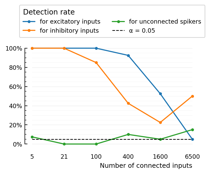
We see monotonic breakdown in excitatory connection detectability.
Same for inhibitory, except it’s not monotonic. Fluke due to sampling?
This plot must be improved with multiple simulations per condition rather than just single point.
(takes a while to run multiple 10’ N=6500 sims though).