2022-02-18 • Scale up N and duration¶

Setup¶

# Pkg.resolve()

include("nb_init.jl")

[ Info: using Revise
[ Info: import Distributions
[ Info: import MyToolbox
[ Info: using VoltageToMap

using Parameters, ComponentArrays
@alias CVec = ComponentVector;

Parameters¶

Simulation duration¶

sim_duration = 1.2 * seconds;

Input spike trains¶

N_unconn = 100
N_exc    = 800
# N_exc    = 5200
N_inh    = N_exc ÷ 4

N_conn = N_inh + N_exc

N = N_conn + N_unconn

input_spike_rate = LogNormal_with_mean(4Hz, √0.6)  # See the previous notebook

LogNormal{Float64}(μ=1.0862943611198905, σ=0.7745966692414834)

Synapses¶

Reversal potential at excitatory and inhibitory synapses, as in the report 2021-11-11__synaptic_conductance_ratio.pdf:

E_exc =   0 * mV
E_inh = -65 * mV;

Synaptic conductances g at t = 0

g_t0 = 0 * nS;

Exponential decay time constant of synaptic conductance, \(τ_{s}\) (s for “synaptic”)

τ_s = 7 * ms;

Increase in synaptic conductance on a presynaptic spike

Δg_exc = 0.1 * nS
Δg_inh = 0.4 * nS;

Izhikevich neuron¶

Initial membrane potential v and adaptation variable u values

v_t0  = -80 * mV
u_t0  =   0 * pA;

Izhikevich’s neuron model parameters for a cortical regular spiking neuron:

cortical_RS = CVec(
    C      = 100 * pF,
    k      = 0.7 * (nS/mV),  # steepness of dv/dt's parabola
    vr     = -60 * mV,
    vt     = -40 * mV,
    a      = 0.03 / ms,      # 1 / time constant of `u`
    b      = -2 * nS,        # how strongly `v` deviations from `vr` increase `u`.
    v_peak =  35 * mV,
    c      = -50 * mV,       # reset voltage.
    d      = 100 * pA,       # `u` increase on spike. Free parameter.
);

Numerics¶

Whether to use a fixed (false) or adaptive timestep (true).

adaptive = true;

Timestep. If adaptive, size of first time step.

dt    = 0.1 * ms;

Minimum and maximum step sizes

dtmax = 0.5  * ms  # solution unstable if not set
dtmin = 0.01 * ms;  # don't spend too much time finding thr crossing or spike arrival

Error tolerances used for determining step size, if adaptive.

The solver guarantees that the (estimated) difference between the numerical solution and the true solution at any time step is not larger than abstol + reltol * |y| (where y ≈ the numerical solution at that time step).

abstol_v = 0.1 * mV
abstol_u = 0.1 * pA
abstol_g = 0.01 * nS;

reltol = 1e-3;  # e.g. if true sol is -80 mV, then max error of 0.08 mV
reltol = 1;     # only use abstol

tol_correction = 0.1;

(abstol_v, abstol_u, abstol_g) .* tol_correction

(1.0e-5, 1.0000000000000002e-14, 1.0000000000000002e-12)

For comparison, the default tolerances for ODEs in DifferentialEquations.jl are

reltol = 1e-2
abstol = 1e-6.

IDs¶

Neuron, synapse & simulated variable IDs.

"""
    idvec(A = 4, B = 2, …)

Build a `ComponentVector` (CVec) with the given group names and
as many elements per group as specified. Each element gets a
unique ID within the CVec, which is also its index in the CVec.
I.e. the above call yields `CVec(A = [1,2,3,4], B = [5,6])`.
Specify `nothing` as size for a scalar element. Example:
`idvec(A=nothing, B=1)` → `CVec(A=1, B=[2])`
"""
function idvec(; kw...)
    cvec = CVec(; (name => _expand(val) for (name, val) in kw)...)
    cvec .= 1:length(cvec)
    return cvec
end;

temp = -1  # value does not matter; they get overwritten by UnitRange
_expand(val::Nothing) = temp
_expand(val::Integer) = fill(temp, val)
_expand(val::CVec)    = val              # allow nested idvecs
;

input_neurons = idvec(conn = idvec(exc = N_exc, inh = N_inh), unconn = N_unconn)

ComponentVector{Int64}(conn = (exc = [1, 2, 3, 4, 5, 6, 7, 8, 9, 10  …  791, 792, 793, 794, 795, 796, 797, 798, 799, 800], inh = [801, 802, 803, 804, 805, 806, 807, 808, 809, 810  …  991, 992, 993, 994, 995, 996, 997, 998, 999, 1000]), unconn = [1001, 1002, 1003, 1004, 1005, 1006, 1007, 1008, 1009, 1010  …  1091, 1092, 1093, 1094, 1095, 1096, 1097, 1098, 1099, 1100])

synapses = idvec(exc = N_exc, inh = N_inh)

ComponentVector{Int64}(exc = [1, 2, 3, 4, 5, 6, 7, 8, 9, 10  …  791, 792, 793, 794, 795, 796, 797, 798, 799, 800], inh = [801, 802, 803, 804, 805, 806, 807, 808, 809, 810  …  991, 992, 993, 994, 995, 996, 997, 998, 999, 1000])

simulated_vars = idvec(v = nothing, u = nothing, g = synapses)

ComponentVector{Int64}(v = 1, u = 2, g = (exc = [3, 4, 5, 6, 7, 8, 9, 10, 11, 12  …  793, 794, 795, 796, 797, 798, 799, 800, 801, 802], inh = [803, 804, 805, 806, 807, 808, 809, 810, 811, 812  …  993, 994, 995, 996, 997, 998, 999, 1000, 1001, 1002]))

Connections¶

postsynapses = Dict{Int, Vector{Int}}()  # input_neuron_ID => [synapse_IDs...]

for (n, s) in zip(input_neurons.conn, synapses)
    postsynapses[n] = [s]
end
for n in input_neurons.unconn
    postsynapses[n] = []
end

Broadcast parameters¶

Δg = similar(synapses, Float64)
Δg.exc .= Δg_exc
Δg.inh .= Δg_inh;

E = similar(synapses, Float64)
E.exc .= E_exc
E.inh .= E_inh;

Initial conditions

vars_t0 = similar(simulated_vars, Float64)
vars_t0.v = v_t0
vars_t0.u = u_t0
vars_t0.g .= g_t0;

Maximum error

abstol = similar(simulated_vars, Float64)
abstol.v = abstol_v
abstol.u = abstol_u
abstol.g .= abstol_g
abstol = abstol .* tol_correction;

ISI distributions¶

Generate firing rates \(λ\) by sampling from the input spike rate distribution.

λ = similar(input_neurons, Float64)
λ .= rand(input_spike_rate, length(λ));
# showsome(λ)

Distributions.jl uses an alternative Exp parametrization, namely scale \(β\) = 1 / rate.

β = 1 ./ λ;

ISI_distributions = similar(input_neurons, Exponential{Float64})
ISI_distributions .= Exponential.(β);

Initialize spiking¶

Generate the first spike time for every input neuron by sampling once from its ISI distribution.

first_spike_times = rand.(ISI_distributions);

Sort these initial spike times by building a priority queue.

upcoming_input_spikes = PriorityQueue{Int, Float64}();

for (neuron, first_spike_time) in enumerate(first_spike_times)
    enqueue!(upcoming_input_spikes, neuron => first_spike_time)
end

`p` object¶

params = (;
    E, Δg, τ_s,
    izh = cortical_RS,
    postsynapses,
    ISI_distributions,
    upcoming_input_spikes,
);

Differential equations¶

The derivative functions that define the differential equations.
Note that discontinuities are defined in the next section.

function f(D, vars, params, _)
    @unpack v, u, g = vars
    @unpack E, τ_s, izh = params
    @unpack C, k, vr, vt, a, b = izh
    I_s = 0.0
    for (gi, Ei) in zip(g, E)
        I_s += gi * (v - Ei)
    end
    D.v = (k * (v - vr) * (v - vt) - u - I_s) / C
    D.u = a * (b * (v - vr) - u)
    D.g .= .-g ./ τ_s
    return nothing
end;

vars = vars_t0
D = similar(vars);

f(D, vars, params, nothing)
@time f(D, vars, params, nothing)

  0.000018 seconds (3 allocations: 128 bytes)

function f2(D,vars,params)
    @unpack v, u, g = vars
    @unpack E, τ_s, izh = params
    @unpack C, k, vr, vt, a, b = izh;
    I_s = 0.0
    for (gi, Ei) in zip(g, E)
        I_s += gi * (v - Ei)
    end
    D.v = (k * (v - vr) * (v - vt) - u - I_s) / C
    D.u = a * (b * (v - vr) - u)
    for i in 1:length(g)
        D.g[i] = -g[i] / τ_s
    end
    return nothing
end;

f2(D,vars,params)
@time f2(D,vars,params)

  0.000010 seconds

nice. so D.g should be loop, for no alloc at all. Even @. didn’t help

Events¶

"""
An `Event` encapsulates two functions that determine when and
how to introduce discontinuities in the differential equations:

- `distance` returns some distance to the next event.
   An event occurs when this distance hits zero.
- `on_event!` is called at each event and may modify
   the simulated variables and the parameter object.

Both functions take the parameters `(vars, params, t)`: the simulated
variables, the parameter object, and the current simulation time.
"""
struct Event
    distance
    on_event!
end;

Input spike generation (== arrival, because no transmission delay):

function time_to_next_input_spike(vars, params, t)
    _, next_input_spike_time = peek(params.upcoming_input_spikes)
    return t - next_input_spike_time
end;

t_ = 0.1s;

time_to_next_input_spike(vars, params, t_)
@time time_to_next_input_spike(vars, params, t_);

  0.000007 seconds (1 allocation: 16 bytes)

The one alloc is for the return value. We hope this function gets inlined where it’s used (condition).

function on_input_spike!(vars, params, t)
    # Process the neuron that just fired.
    # Start by removing it from the queue.
    fired_neuron = dequeue!(params.upcoming_input_spikes)
    
    # Generate a new spike time, and add it to the queue.
    new_spike_time = t + rand(params.ISI_distributions[fired_neuron])
    enqueue!(params.upcoming_input_spikes, fired_neuron => new_spike_time)
    
    # Update the downstream synapses
    # (number of these synapses in the N-to-1 case: 0 or 1).
    for synapse in params.postsynapses[fired_neuron]
        vars.g[synapse] += params.Δg[synapse]
    end

end

input_spike = Event(time_to_next_input_spike, on_input_spike!);

on_input_spike!(vars, params, t_)
@time on_input_spike!(vars, params, t_);

  0.000019 seconds

Nice! no allocs already

Spike threshold crossing of Izhikevich neuron

distance_to_v_peak(vars, params, _) = vars.v - params.izh.v_peak;

distance_to_v_peak(vars, params, t_)
@time distance_to_v_peak(vars, params, t_);

  0.000005 seconds (1 allocation: 16 bytes)

same thang, return val.

function on_v_peak!(vars, params, _)
    # The discontinuous LIF/Izhikevich/AdEx update
    vars.v = params.izh.c
    vars.u += params.izh.d
    return nothing
end

spiking_threshold_crossing = Event(distance_to_spiking_threshold, on_spiking_threshold_crossing!);

on_v_peak!(vars, params, t_)
@time on_v_peak!(vars, params, t_);

  0.000006 seconds

I added return nothing so no alloc.

events = [input_spike, spiking_threshold_crossing];

diffeq.jl API¶

Set-up problem and solution in DifferentialEquations.jl’s API.

@withfeedback using OrdinaryDiffEq

[ Info: using OrdinaryDiffEq

prob = ODEProblem(f, vars_t0, float(sim_duration), params);

function condition(distance, vars, t, integrator)
    for (i, event) in enumerate(events)
        distance[i] = event.distance(vars, integrator.p, t)
    end
end;

distance = zeros(2)
integrator = (p = params,);

condition(distance, vars, t_, integrator)
@time condition(distance, vars, t_, integrator);

  0.000014 seconds (19 allocations: 624 bytes)

integrator = (;params, events);

function c2(distance, vars, t, int)
    for i in 1:10 end   # no alloc
    # for i in 1:length(events) end  # 3 allocs!! 100 byte
    for i in 1:length(int.events) end  # no alloc :)   (thanks to no global)
    for (i, event) in enumerate(int.events)
        # distance[i] = event.distance(vars, int.params, t)  # 8 allocs, 256 bytes
    end
end;

c2(distance, vars, t_, integrator)
@time c2(distance, vars, t_, integrator);

  0.000012 seconds (8 allocations: 256 bytes)

@time events[1].distance(vars, integrator.params, t_);

  0.000018 seconds (5 allocations: 240 bytes)

@time events[1].distance(vars, params, t_);

  0.000013 seconds (3 allocations: 80 bytes)

@time time_to_next_input_spike(vars, params, t_);

  0.000007 seconds (1 allocation: 16 bytes)

function affect!(integrator, i)
    events[i].on_event!(integrator.u, integrator.p, integrator.t)
end

callback = VectorContinuousCallback(condition, affect!, length(events));

solver = Tsit5()

Tsit5(stage_limiter! = trivial_limiter!, step_limiter! = trivial_limiter!, thread = static(false))

save_idxs = [simulated_vars.v, simulated_vars.u];

progress = true;

solve_() = solve(
    prob, solver;
    callback, save_idxs, progress,
    adaptive, dt, dtmax, dtmin, abstol, reltol,
);

Solve¶

sol = @time solve_();

 16.172403 seconds (24.21 M allocations: 1.162 GiB, 5.96% gc time, 88.36% compilation time)

sol = @time solve_();

 12.388856 seconds (23.88 M allocations: 1.152 GiB, 4.50% gc time, 89.20% compilation time)

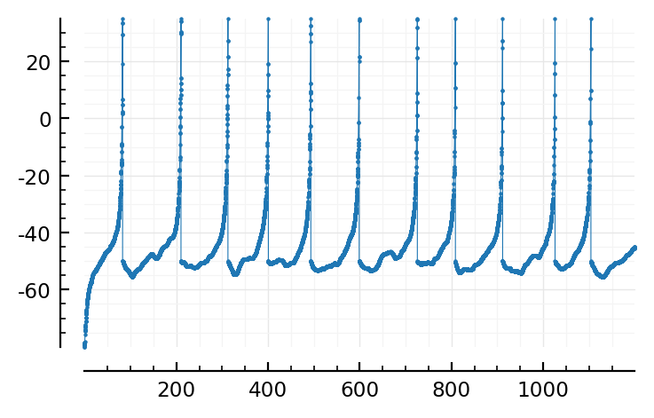
Plot¶

@withfeedback import PyPlot
using Sciplotlib

[ Info: import PyPlot

""" t = [200ms, 600ms] e.g. """
function Sciplotlib.plot(sol::ODESolution; t = nothing)
    isnothing(t) && (t = sol.t[[1,end]])
    izoom = first(t) .< sol.t .< last(t)
    plot(
        sol.t[izoom] / ms,
        sol[1,izoom] / mV,
        clip_on = false,
        marker = ".", ms = 1.2, lw = 0.4,
        #  xlim = t,  # haha lolwut, adding this causes fig to no longer display.
    )
end;

plot(sol);

../_images/2022-02-18__scale_up_N_and_duration_120_0.png

Voltage-to-Wiring Sim

2022-02-18 • Scale up N and duration

Contents

2022-02-18 • Scale up N and duration¶

Setup¶

Parameters¶

Simulation duration¶

Input spike trains¶

Synapses¶

Izhikevich neuron¶

Numerics¶

IDs¶

Connections¶

Broadcast parameters¶

ISI distributions¶

Initialize spiking¶

`p` object¶

Differential equations¶

Events¶

diffeq.jl API¶

Solve¶

Plot¶

Voltage-to-Wiring Sim

2022-02-18 • Scale up N and duration

Contents

2022-02-18 • Scale up N and duration¶

Setup¶

Parameters¶

Simulation duration¶

Input spike trains¶

Synapses¶

Izhikevich neuron¶

Numerics¶

IDs¶

Connections¶

Broadcast parameters¶

ISI distributions¶

Initialize spiking¶

p object¶

Differential equations¶

Events¶

diffeq.jl API¶

Solve¶

Plot¶

`p` object¶