2020-11-27 • Permutation test for p(connected)
Contents
2020-11-27 • Permutation test for \(p(\)connected\()\)
Imports & time grid
from voltage_to_wiring_sim.support.notebook_init import *
Preloading:
 - numpy … (0.19 s)
 - matplotlib.pyplot … (0.30 s)
 - numba … (0.45 s)

Importing from submodules (compiling numba functions) … ✔

Imported `np`, `mpl`, `plt`
Imported codebase (`voltage_to_wiring_sim`) as `v`
Imported `*` from `v.support.units`
Setup autoreload
v.print_reproducibility_info()
This cell was last run by tfiers on yoga
on Mon 30 Nov 2020, at 15:59 (UTC+0100).
Last git commit (Mon 30 Nov 2020, 12:19).
Uncommited changes to:
A notebooks/2020-11-11__unitlib.ipynb
tg = v.TimeGrid(T=10*minute, dt=0.1*ms);
Generate VI signal
Spike trains
‘Network’ definition.
N_in = 30
p_connected = 0.5

N_connected = round(N_in * p_connected)
N_unconnected = N_in - N_connected
15
Have all incoming neurons spike with the same mean frequency, for now.
f_spike = 20 * Hz;
gen_st = v.generate_Poisson_spike_train

v.fix_rng_seed()
%%time
spike_trains_connected = [gen_st(tg, f_spike) for _ in range(N_connected)]
spike_trains_unconnected = [gen_st(tg, f_spike) for _ in range(N_unconnected)];
Wall time: 1.95 s
all_spike_trains = spike_trains_connected + spike_trains_unconnected;
Inspect a time excerpt..
time_slice = 1 * minute + np.array([0, 1]) * second

slice_indices = np.round(time_slice / tg.dt).astype(int)
i_slice = slice(*slice_indices)
t_slice = tg.t[i_slice]
array([60, 60, 60, ..., 61, 61, 61])
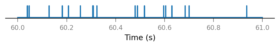
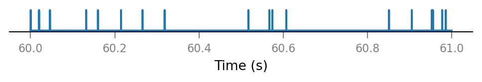
..of one presynaptic neuron:
def plot_spike_train_excerpt(spike_train):
    return v.spike_train.plot(t_slice, spike_train[i_slice])
plot_spike_train_excerpt(all_spike_trains[0]);
All connected presynaptic neurons:
all_incoming_spikes = sum(spike_trains_connected)

v.spike_train.plot(t_slice, all_incoming_spikes[i_slice]);
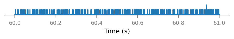
Note that some time bins contain more than one spike.
(The simulator handles this, by increasing synaptic conductance by an integer multiple of Δg_syn in that timebin).
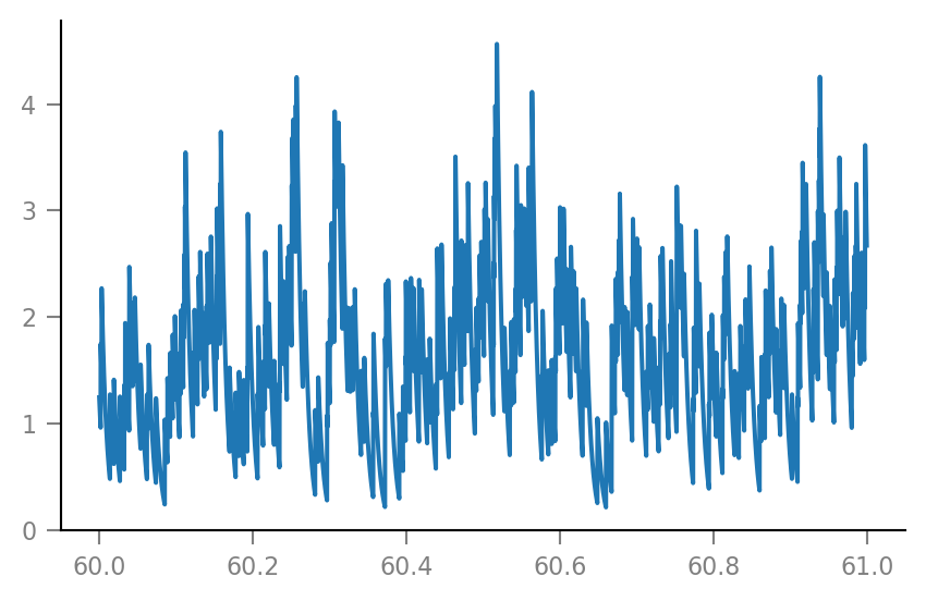
Synaptic conductance
See the previous notebook /notebooks/2020-07-27__Synaptic_conductances for some more explanation.
Δg_syn = 0.8 * nS
τ_syn = 7 * ms;
g_syn = v.calc_synaptic_conductance(
    tg, all_incoming_spikes, Δg_syn, τ_syn)

plt.plot(t_slice, g_syn[i_slice] / nS);
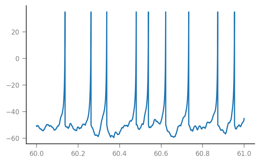
Membrane voltage
params = v.params.cortical_RS
v.pprint(params)
IzhikevichParams
----------------
C = 1e-10
k = 7e-07
v_r = -0.06
v_t = -0.04
v_peak = 0.035
a = 30.0
b = -2e-09
c = -0.05
d = 1e-10
v_syn = 0.0
%%time
sim = v.simulate_izh_neuron(tg, params, g_syn)
Wall time: 246 ms
plt.plot(t_slice, sim.V_m[i_slice] / mV);
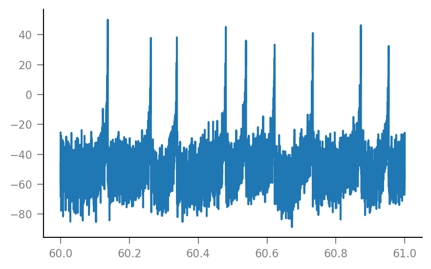
Imaging model
As in /notebooks/2020-07-06__Single_neuron_sim.
Vm_noisy = v.add_VI_noise(sim.V_m, params)

plt.plot(t_slice, Vm_noisy[i_slice] / mV);
Shuffle one spike train
We choose one spike train / incoming neuron, and will test the hypothesis that this neuron is connected to the simulated neuron.
H0 = neuron of incoming spike train is not connected to simulated neuron
H1 = they are connected
spike_train = all_spike_trains[0];
We will shuffle the real spike train \(S\) times to generate \(S\) ‘fake’ spike trains, which have the same number of spikes but at random times.
S = 100;
%%time
shuffled_spike_trains = []
for i in range(S):
    x = spike_train.copy()
    np.random.shuffle(x)  # in-place
    shuffled_spike_trains.append(x)
Wall time: 23.4 s
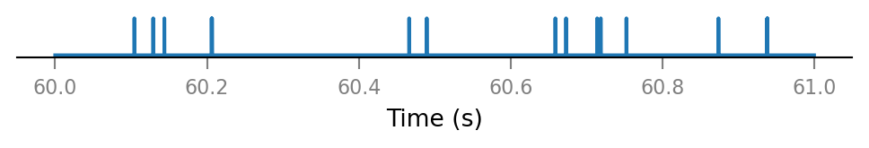
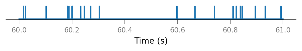
Inspect a few shuffled spike trains.
for i in range(3):
    plot_spike_train_excerpt(shuffled_spike_trains[i]);
Real spike train again:
plot_spike_train_excerpt(spike_train);

Same number of spikes in all:
def num_spikes(spike_train):
    spike_indices = v.get_spike_indices(spike_train)
    return len(spike_indices)
for i in range(3):
    print(num_spikes(shuffled_spike_trains[i]))
12020
12020
12020
num_spikes(spike_train)
12020
Spiking frequency of the chosen presynaptic neuron:
num_spikes(spike_train) / tg.T / Hz
20.03
That’s to spec.
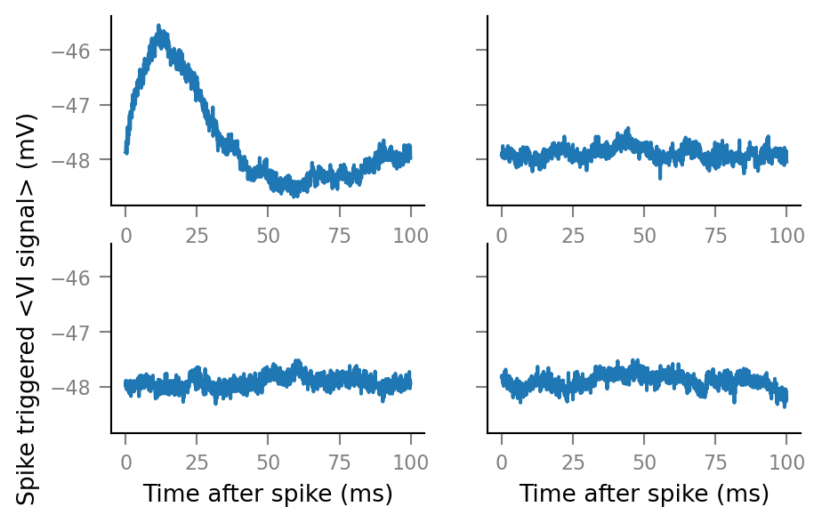
Spike-triggered windowing & averaging
For each spike train (original and shuffleds), we extract spike-triggered windows from the simulated voltage imaging signal, and average those windows.
window_length = 100 * ms;
window_tg = v.TimeGrid(window_length, tg.dt);
def calc_STA(spike_train):
    return v.calculate_STA(Vm_noisy, spike_train, tg, window_tg)
original_STA = calc_STA(spike_train);
%%time
shuffled_STAs = []
for train in shuffled_spike_trains:
    shuffled_STAs.append(calc_STA(train))
Wall time: 9.14 s
Plot STA’s of the original spike train (top left) and three shuffled spike trains:
fig, axes = plt.subplots(ncols=2, nrows=2, sharey=True)

original_ax = axes.flat[0]
v.plot_STA(original_STA, window_tg, original_ax)
ylabel = original_ax.yaxis.get_label()
ylabel.set_horizontalalignment('right')


for i in range(3):
    ax = axes.flat[i+1]
    v.plot_STA(shuffled_STAs[i], window_tg, ax)
    ax.set(ylabel=None)
Peak height of STA
shuffled_STA_peak_heights = []
for STA in shuffled_STAs:
    shuffled_STA_peak_heights.append(np.max(STA))
shuffled_STA_peak_heights = np.array(shuffled_STA_peak_heights);
    # Convert list to numpy array for division or comparison with scalars later.
original_STA_peak_height = np.max(original_STA);
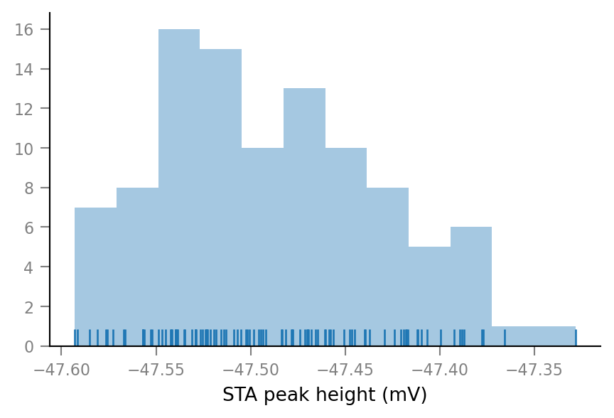
Let’s look at the distribution of peak heights.
import seaborn as sns # Extension of matplotlib for statistical data viz.
Shuffled spike trains only:
dist_ax = sns.distplot(shuffled_STA_peak_heights / mV, kde=False, rug=True, bins=12)
#   KDE=False means that the y-axis labels give count in each bin. (Otherwise, it's a density).
dist_ax.set_xlabel("STA peak height (mV)");
Add original spike train:
dist_ax.axvline(original_STA_peak_height / mV, color="C1")
dist_ax.figure
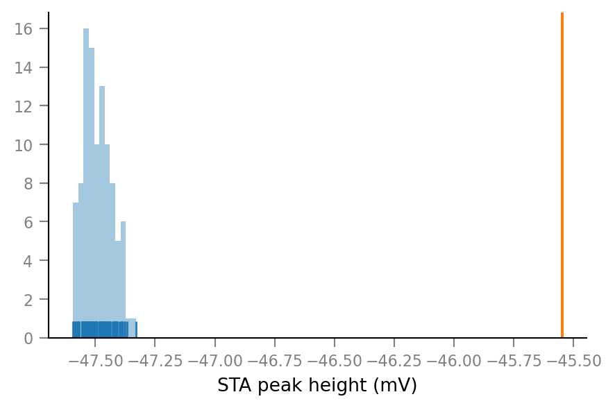
p-value
As proportion
If we define p-value as proportion of shuffled STA peak heights higher than the original, we get, of course:
p_proportion = np.sum(shuffled_STA_peak_heights > original_STA_peak_height) / S
0.0
(As integral of KDE)
We can fit a distribution to the H0 peak heights to get another type of p-value.
We choose a kernel-density estimate (KDE), i.e. a non-paramteric distribution (except hyperparams). (See here for code explanation: https://jakevdp.github.io/PythonDataScienceHandbook/05.13-kernel-density-estimation.html#Kernel-Density-Estimation-in-Practice)
from sklearn.neighbors import KernelDensity
kde = KernelDensity(kernel='gaussian', bandwidth=0.1 * mV)
kde.fit(shuffled_STA_peak_heights[:, np.newaxis])  # `fit` expects 2D array.

def plot_KDE(xrange):  # xrange given in mV
    x = np.linspace(*np.array(xrange) * mV, 1000)[:, np.newaxis]
    y = np.exp(kde.score_samples(x));  # `score_samples` returns log of prob.
    fig, ax = plt.subplots()
    ax.plot(x / mV, y)
    ax.axvline(original_STA_peak_height / mV, color="C1")
    return fig, ax

plot_KDE(dist_ax.get_xlim());
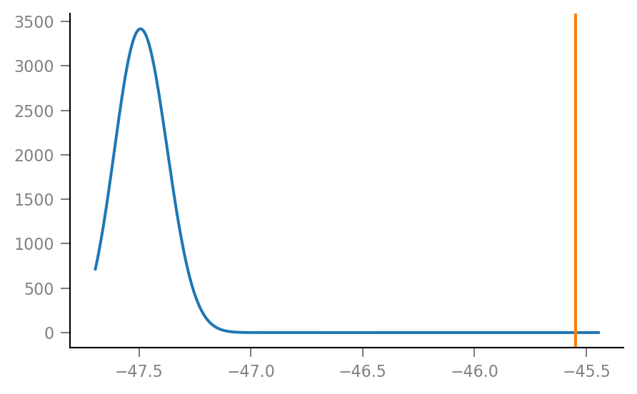
plot_KDE((-45.6, -45.5));
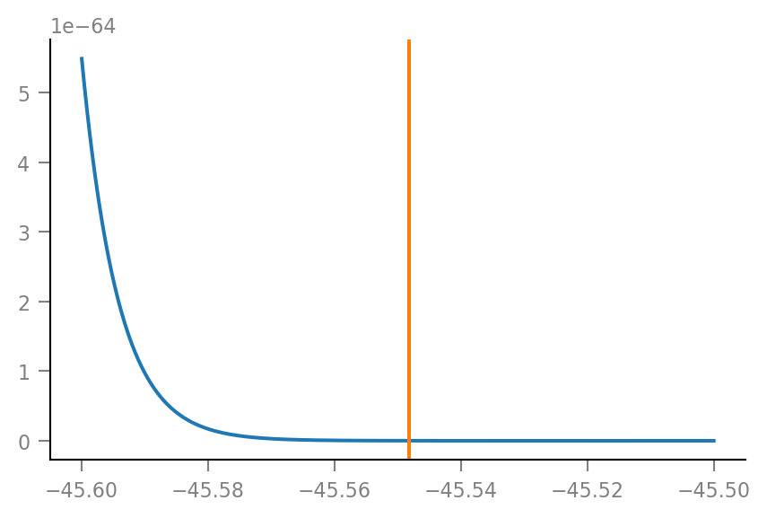
def pdf(x):
    return np.exp(kde.score_samples([[x]])).item()

pdf(original_STA_peak_height)
6.209E-68
p-value is area under the curve to the right of original spike train peak STA height.
from scipy.integrate import quad
Docs: https://docs.scipy.org/doc/scipy/reference/generated/scipy.integrate.quad.html
result, error = quad(pdf, a=original_STA_peak_height, b=0 * mV)
(result, error)
(1.099E-75, 2.186E-75)
The absolute error is larger than the estimated integral. The result is thus not reliable.
Anyway, from the plots it’s clear that this p-value is very small.
Next steps: describe influence of N_in, p_connected, SNR, … on p-value.
repeat for all connected/unconnected spike trains
Some feedback from code review
(see also supervision record 30th nov).
Three stages of pipeline:
neuron model
VI model
test
Noise both for neuron and for inputs.
Lit on statistics of non-recorded spike trains noise
p < 0.01
1/S
0.01
Repro info
v.print_reproducibility_info(verbose=True)
This cell was last run by tfiers on yoga
on Mon 30 Nov 2020, at 16:01 (UTC+0100).
Last git commit (Mon 30 Nov 2020, 12:19).
Uncommited changes to:
A  notebooks/2020-11-11__unitlib.ipynb
 M notebooks/2020-11-27__permutation_test.ipynb
Platform:
Windows-10
CPython 3.8.3 (C:\conda\python.exe)
Intel(R) Core(TM) i7-10510U CPU @ 1.80GHz
Dependencies of voltage_to_wiring_sim and their installed versions:
numpy                1.19.2
matplotlib           3.3.2
numba                0.51.2
seaborn              0.10.1
scipy                1.5.2
scikit-learn         0.23.2
preload              2.1
py-cpuinfo           7.0.0