2022-09-15 • Two-pass connection test: ptp, then corr with found avg¶

Two-pass connection test: peak-to-peak, then correlation with found average

Imports¶

using MyToolbox

using VoltoMapSim

[ Info: Precompiling VoltoMapSim [f713100b-c48c-421a-b480-5fcb4c589a9e]

Params¶

p = get_params(
    duration = 10minutes,
    p_conn = 0.04,
    g_EE = 1,
    g_EI = 1,
    g_IE = 4,
    g_II = 4,
    ext_current = Normal(-0.5 * pA/√seconds, 5 * pA/√seconds),
    E_inh = -80 * mV,
    record_v = [1:40; 801:810],
);

Run sim¶

@time s = cached(sim, [p.sim]);

Loading cached output from `C:\Users\tfiers\.phdcache\datamodel v2 (net)\sim\ce5e30aee45561ed.jld2` … done (8.6 s)
  9.992754 seconds (12.06 M allocations: 3.025 GiB, 9.21% gc time, 69.41% compilation time: 5% of which was recompilation)

@time s = augment(s, p);

  2.605456 seconds (4.91 M allocations: 293.675 MiB, 8.31% gc time, 97.97% compilation time: 1% of which was recompilation)

1. peak-to-peak¶

We take all inputs with predicted_type :exc.

Current pval threshold is 0.05.
We could be stricter.

It’ll be tradeoff: stricter threshold gives less STAs to average to build our template; but there will be less noisy STAs mixed in (or even wrong STAs, i.e. of non-inputs).

Now

Get the :exc input detections for neuron 1
Average their STA
Apply this template to STAs of all inputs

# But first: cache STAs :)

Construct ‘tested_connections’ table¶

SimData = typeof(s);

function get_tested_connections(s::SimData, p::ExpParams)
    # We do not test all N x N connections (that's too much).
    # The connections we do test are determined by which neurons
    # we record the voltage of, and the `N_tested_presyn` parameter.
    
    tested_connections = DataFrame(
        post     = Int[],     # neuron ID  
        pre      = Int[],     # neuron ID
        conntype = Symbol[],  # :exc or :inh or :unconn
        posttype = Symbol[],  # :exc or :inh
    )
    
    @unpack N_tested_presyn, rngseed = p.conntest
    
    resetrng!(rngseed)
    
    function get_labelled_sample(input_neurons, conntype)
        # Example output: `[(3, :exc), (5, :exc), (12, :exc), …]`.
        N = min(length(input_neurons), N_tested_presyn)
        inputs_sample = sample(input_neurons, N, replace = false, ordered = true)
        zip(inputs_sample, fill(conntype, N))
    end
    
    recorded_neurons = keys(s.v) |> collect |> sort!
    
    for post in recorded_neurons
        
        posttype = s.neuron_type[post]
        
        inputs_to_test = chain(
            get_labelled_sample(s.exc_inputs[post], :exc),
            get_labelled_sample(s.inh_inputs[post], :inh),
            get_labelled_sample(s.non_inputs[post], :unconn),
        ) |> collect
        
        for (pre, conntype) in inputs_to_test
            push!(tested_connections, (; post, pre, conntype, posttype))
        end
    end
    
    return tested_connections
end

tc = get_tested_connections(s, p)

disp(tc, 3)

3,906 rows × 4 columns

	post	pre	conntype	posttype
	Int64	Int64	Symbol	Symbol
1	1	139	exc	exc
2	1	681	exc	exc
3	1	11	exc	exc
&vellip;	&vellip;	&vellip;	&vellip;	&vellip;

Calc all STAs¶

using Base.Threads

function calc_all_STAs(s::SimData, p::ExpParams)
    # Multi-threaded calculation of the real and shuffled STAs of all tested connections.
    #
    # We use a Channel to gather calculations,
    # as inserting items into a Dict is not thread-safe.
    @unpack rngseed, num_shuffles = p.conntest
    tc = tested_connections = get_tested_connections(s, p)
    recorded_neurons = unique(tested_connections.post)
    ch = Channel(Inf)  # `Inf` size, so no blocking on insert
    @info "Using $(nthreads()) threads"
    pbar = Progress(nrow(tested_connections), desc = "Calculating STAs: ")
    @threads(
    for m in recorded_neurons
        v = s.v[m]
        inputs_to_test = tc.pre[tc.post .== m]
        for n in inputs_to_test
            spikes = s.spike_times[n]
            real_STA = calc_STA(v, spikes, p)
            shuffled_STAz = Vector(undef, num_shuffles)  # [1]
            resetrng!(rngseed)
            for i in 1:num_shuffles
                shuffled_spikes = shuffle_ISIs(spikes)
                shuffled_STAz[i] = calc_STA(v, shuffled_spikes, p)
            end
            put!(ch, ((n => m), real_STA, shuffled_STAz))
            next!(pbar)
        end
    end)
    # Empty the channel, into the output dicts
    STAs          = Dict{Pair{Int, Int}, Vector{Float64}}()
    shuffled_STAs = Dict{Pair{Int, Int}, Vector{Vector{Float64}}}()
    while !isempty(ch)
        conn, real, shuffleds = take!(ch)
        STAs[conn]          = real
        shuffled_STAs[conn] = shuffleds
    end
    close(ch)
    
    return (; tested_connections, STAs, shuffled_STAs)
end

# [1] Giving this the same name as the output dict, in combination with `@threads`,
#     confuses type inference and makes it infer `Any` for the `shuffled_STAs` output dict.
#     (That doesn't matter though, as this is a user-facing, top-level function; not an inner-loop one).

calc_all_STAs (generic function with 1 method)

# For 4000 connections tested (0.4% of all) and 100 shuffles,
# we get 404_000 STAs.
# At 1000 Float64 samples per STA, that is 3.2 GB.

# On typing (code_warntype) of calc_all_STAs:
# it didn't matter for timing it was untyped
# (tested with small params `q`, 447 conns).

out = cached(calc_all_STAs, [s,p], key=[p.sim, p.conntest]);

[ Info: Using 7 threads
Calculating STAs: 100%|█████████████████████████████████| Time: 0:19:04
Saving output at `C:\Users\tfiers\.phdcache\datamodel v2 (net)\calc_all_STAs\b9353bdd11d8b8cb.jld2` … done (18.2 s)

@time (out = cached(calc_all_STAs, [s,p], key=[p.sim, p.conntest]));

Loading cached output from `C:\Users\tfiers\.phdcache\datamodel v2 (net)\calc_all_STAs\b9353bdd11d8b8cb.jld2` … done (19.3 s)
 19.725458 seconds (9.35 M allocations: 3.348 GiB, 28.71% gc time, 10.98% compilation time)

tested_connections, STAs, shuffled_STAs = out;

Calc pval¶

Sig = Vector{Float64}

function calc_pval(real_STA::Sig, shuffled_STAs::Vector{Sig}, test_stat)
    real_t      = test_stat(real_STA)
    shuffled_ts = [test_stat(STA) for STA in shuffled_STAs]
    num_shuffled_larger = count(shuffled_ts .> real_t)
    N = length(shuffled_STAs)
    return if num_shuffled_larger == 0
        (pval      = 1/N,
         pval_type = "<")
    else
        (pval      = num_shuffled_larger / N,
         pval_type = "=")
    end
end

calc_pval (generic function with 1 method)

Test connections¶

function test_conn__ptp((from,to), STAs, shuffled_STAs; α)
    # α is the p-value threshold.
    pval, _ = calc_pval(STAs[from=>to], shuffled_STAs[from=>to], ptp)
    area = area_over_start(STAs[from=>to])
    if (pval > α)      predtype = :unconn
    elseif (area > 0)  predtype = :exc
    else               predtype = :inh    end
    return (; predtype, pval, area)
end;

test_conn__ptp((from,to); α) = test_conn__ptp((from,to), STAs, shuffled_STAs; α);

test_conn__ptp(139=>1, α = 0.01)

(predtype = :exc, pval = 0.01, area = 0.16991151700597443)

testresults = 
    @showprogress "Testing connections: " (
    map(eachrow(tested_connections)) do r
        test_conn__ptp(r.pre => r.post, α = 0.01)
    end
);

Testing connections: 100%|██████████████████████████████| Time: 0:00:04

tc = hcat(tested_connections, DataFrame(testresults))
select!(tc, :posttype, :post, :pre, :conntype, :predtype, :pval, :area)
disp(tc, 3)

3,906 rows × 7 columns

	posttype	post	pre	conntype	predtype	pval	area
	Symbol	Int64	Int64	Symbol	Symbol	Float64	Float64
1	exc	1	139	exc	exc	0.01	0.169912
2	exc	1	681	exc	unconn	0.02	-0.0399586
3	exc	1	11	exc	exc	0.01	0.180399
&vellip;	&vellip;	&vellip;	&vellip;	&vellip;	&vellip;	&vellip;	&vellip;

(“predtype” is predicted conntype).

We used strict α of 0.01.

Out of interest, what is the T and FPR.

Detection rates¶

Previously, we had detection rates per recorded (‘post’) neuron. We can also just calculate the rates over the whole table. Corresponds to the mean of previous notebooks.

detrate(typ) = count((tc.conntype .== typ) .& (tc.predtype .== typ)) / count(tc.conntype .== typ)

(
    TPR_exc = detrate(:exc),
    TPR_inh = detrate(:inh),
    FPR = 1 - detrate(:unconn),
)

(TPR_exc = 0.521, TPR_inh = 0.831, FPR = 0.0785)

We’ll use E→E connections for our template.

How many of these did we detect,
and how many of the detected are false.

# so we search for [posttype=:exc],
# and then - [conntype=:exc, predtpye=:exc]
#          - [conntype=:unconn, predtype=:exc]

This is precision, not TPR (aka accuracy).

Precision¶

using DataFramesMeta

df = tc[tc.posttype .== :exc, :]

precision = count((df.predtype .== :exc) .& (df.conntype .== :exc)) / count(df.predtype .== :exc)

0.925

num_EE_detections = count(df.predtype .== :exc)

correct_EE_detections = precision * num_EE_detections

incorrect_EE_detections = (1 - precision) * num_EE_detections

Note that this presumes we know the type of each neuron (‘post’).

Yeah that’s not general.

Let’s instead just take all exc detected connections, whether or not post is exc or inh.

..of all detected exc connections¶

(So also exc→inh)

# sub back df > tc
precision = count((tc.predtype .== :exc) .& (tc.conntype .== :exc)) / count(tc.predtype .== :exc)

0.934

num_exc_detections = count(tc.predtype .== :exc)

correct_exc_detections = precision * num_exc_detections

incorrect_exc_detections = (1 - precision) * num_exc_detections

So to summarize, we detected 52% of true exc connections,
and 93% of what we detected as exc is actually exc.

2. STA template¶

det_exc_conns = [r.pre=>r.post for r in eachrow(tc) if r.predtype == :exc];

template_ptp = mean(STAs[c] for c in det_exc_conns);

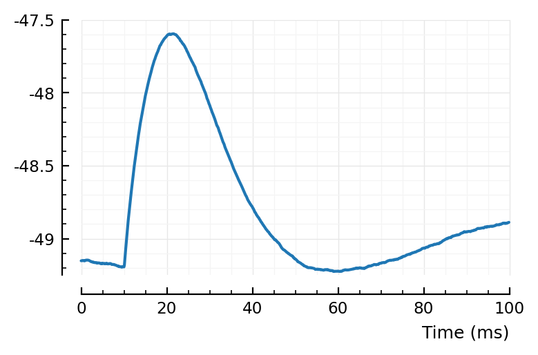
plotsig(template_ptp / mV, p);

../_images/2022-09-15__Two-pass_conntest_ptp-then-cor_57_0.png

# now to corr this, for all conns.

function test_conn__corr((from,to), STAs, shuffled_STAs; α, template)
    # α is the p-value threshold.
    STA = STAs[from=>to]
    corr = cor(STA, template)

    if (corr > 0) test_stat = (STA -> cor(STA, template))
    else          test_stat = (STA -> -cor(STA, template)) end

    pval, _ = calc_pval(STA, shuffled_STAs[from=>to], test_stat)
    if     (pval > α)  predtype = :unconn
    elseif (corr > 0)  predtype = :exc
    else               predtype = :inh end
    return (; predtype, pval, corr)
end
# note: closure of `template`

test_conn__corr((from,to)                     ; α, template = template_ptp) =
test_conn__corr((from,to), STAs, shuffled_STAs; α, template);

function test_conns(testfunc; α)
    testresults = 
        @showprogress "Testing connections: " (
        map(eachrow(tested_connections)) do r
            testfunc(r.pre => r.post; α)
        end)
    
    tc = hcat(tested_connections, DataFrame(testresults))
    
    # Reorder first cols:
    select!(tc, :posttype, :post, :pre, :conntype, :)
    
    num_TP(typ) = count((tc.conntype .== typ) .& (tc.predtype .== typ))
    num_real(typ)     = count(tc.conntype .== typ)
    num_detected(typ) = count(tc.predtype .== typ)
    
    TPR(typ)       = num_TP(typ) / num_real(typ)
    precision(typ) = num_TP(typ) / num_detected(typ)
    
    perf = (
        TPR_exc     = TPR(:exc),
        TPR_inh     = TPR(:inh),
        FPR         = 1 - TPR(:unconn),
        prec_exc    = precision(:exc),
        prec_inh    = precision(:inh),
        prec_unconn = precision(:unconn),
    )
    return (; tc, perf)
end

res_2pass = test_conns(test_conn__corr, α = 0.05);

Testing connections: 100%|██████████████████████████████| Time: 0:00:01

Note α = 5% here; in the ptp step, it was the stricter 1%.

res_2pass.perf

(TPR_exc = 0.8151815181518152, TPR_inh = 0.9360613810741688, FPR = 0.14800000000000002, prec_exc = 0.8988355167394468, prec_inh = 0.6918714555765595, prec_unconn = 0.8507239141288068)

(Note that TPR no longer broken down by postsynaptic type here. Also, we added precision as performance measure: how much of detected are correct).

Compare performance¶

..with just ptp-and-area, now with α = 0.05 too:

res_ptp = test_conns(test_conn__ptp, α = 0.05);

Testing connections: 100%|██████████████████████████████| Time: 0:00:01

To compare with the previous correlation-test-notebook, where we cheated by using the average STA of all a-priori known E→E connections as template, ..

..we used different measure there (calculate detection rates per postsynaptic neuron, and then take the median of that. Also these rates were broken down by postsyn type). The measures here are simpler.

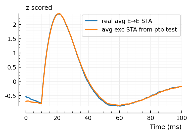
EE_conns = [r.pre=>r.post for r in eachrow(tc) if (r.conntype == :exc) & (r.posttype .== :exc)];

avg_EE_STA = mean(STAs[c] for c in EE_conns);

plotsig(zscore(avg_EE_STA), p, label = "real avg E→E STA");
plotsig(zscore(template_ptp), p, label = "avg exc STA from ptp test", hylabel="z-scored")
plt.legend();
# zscore, as ptp template has larger range (hm!)

../_images/2022-09-15__Two-pass_conntest_ptp-then-cor_70_0.png

We should not calc the real E→E STA to compare,
but rather the E→any STA.

exc_conns = [r.pre=>r.post for r in eachrow(tc) if (r.conntype == :exc)];
avg_exc_STA = mean(STAs[c] for c in exc_conns);

plotsig(zscore(avg_exc_STA), p, label = "real avg exc STA");
plotsig(zscore(template_ptp), p, label = "avg exc STA from ptp test", hylabel="z-scored")
plt.legend();

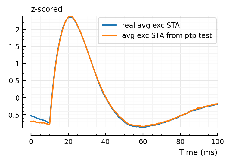
../_images/2022-09-15__Two-pass_conntest_ptp-then-cor_73_0.png

Not a large difference it seems (not identical either).

Also interesting that the ptp STA has a larger range than the real avg STA:

plotsig(avg_exc_STA / mV, p, label = "real avg exc STA");
plotsig(template_ptp / mV, p, label = "avg exc STA from ptp test", hylabel="mV")
plt.legend();

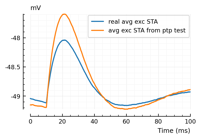
../_images/2022-09-15__Two-pass_conntest_ptp-then-cor_75_0.png

Ah of course: reason why real average STA is smaller, is cause it also includes weaker connections, which the strict ptp test did not pick up.

# Now use this real avg STA as template

testfunc(conn; α) = test_conn__corr(conn; α, template = avg_exc_STA);

res_real_avg = test_conns(testfunc, α = 0.05);

Testing connections: 100%|██████████████████████████████| Time: 0:00:00

res_real_avg.perf

(TPR_exc = 0.8145214521452145, TPR_inh = 0.9360613810741688, FPR = 0.14700000000000002, prec_exc = 0.8981077147016011, prec_inh = 0.6958174904942965, prec_unconn = 0.8504486540378864)

df = DataFrame([
        (; method="ptp only",         res_ptp.perf...),
        (; method="ptp-then-corr",    res_2pass.perf...),
        (; method="corr w/ real avg", res_real_avg.perf...),
    ]
);

Summary table¶

printsimple(df)

 method            TPR_exc  TPR_inh  FPR    prec_exc  prec_inh  prec_unconn 
────────────────────────────────────────────────────────────────────────────
 ptp only          0.574    0.849    0.145  0.889     0.466     0.772
 ptp-then-corr     0.815    0.936    0.148  0.899     0.692     0.851
 corr w/ real avg  0.815    0.936    0.147  0.898     0.696     0.85

So the two-pass connection test idea works well – very nearly as well as the ‘cheating’ test where we correlate with the real average excitatory STA (instead of an average STA found after a first-pass, strict peak-to-peak test).

On what the numbers mean:

FPR is how many non-connections were classified as connected.

85% precision_unconn means that 15% of what we said was not connected actually was.

By also calculating precision (aka positive predictive value) as a performance measure, we see that our high inhibitory detection rates trade-off against a lower precision, compared to excitatory connections.

Confusion matrix¶

..with counts, and ratios too.

function calc_perf_measures(tc::DataFrame)
    # `tc` is a `tested_connections` table with `predtype` (prediction) column added.
    conntypes = [:unconn, :exc, :inh]
    conntypes_matrix = [(pred, real) for pred in conntypes, real in conntypes]
    counts = similar(conntypes_matrix, Int)  # Detection counts
    for (i, (pred, real)) in enumerate(conntypes_matrix)
        counts[i] = count((tc.predtype .== pred) .& (tc.conntype .== real))
    end
    N = length(conntypes)
    sensitivities  = Vector(undef, N)  # aka TPRs
    precisions     = Vector(undef, N)
    for i in 1:N
        num_correct   = counts[i,i]
        num_real      = sum(counts[:,i])
        num_predicted = sum(counts[i,:])
        sensitivities[i] = num_correct / num_real
        precisions[i]    = num_correct / num_predicted
    end
    return (; counts, sensitivities, precisions, conntypes, conntypes_matrix)
end;

function make_perf_display(tested_connections::DataFrame)
    
    data = calc_perf_measures(tested_connections)
    
    titlerow = titlecol = 1
    grouprow = groupcol = 2
    datarows = datacols = 3:5
    sens_row = prec_col = 7
    nrows    = ncols    = 7

    cells = Matrix{Any}(undef, nrows, ncols)
    fill!(cells, "")

    cells[grouprow, datacols] .= data.conntypes
    cells[datarows, groupcol] .= data.conntypes
    cells[datarows, datacols] .= data.counts

    cells[datarows, titlecol] .= [
        "             ┌",
        "Predicted type",
        "             └",
    ]
    cells[titlerow, datacols] .= ["┌───────", "Real type", "───────┐"]

    fmt_pct(x) = join([round(Int, 100x), "%"])
    cells[sens_row, titlecol]  = "Sensitivity"
    cells[sens_row, datacols] .= fmt_pct.(data.sensitivities)
    cells[titlerow, prec_col]  = "Precision"
    cells[datarows, prec_col] .= fmt_pct.(data.precisions)

    title = join(["Tested connections: ", sum(data.counts)])
    
    bold_cells = vcat([(titlerow,c) for c in 1:ncols], [(r,titlecol) for r in 1:nrows])

    return DisplayTable(cells, title, bold_cells)
end;

(I made displaytable.jl in ../pkg/MyToolbox/src/)

t = make_perf_display(res_2pass.tc);
print(t)

Tested connections: 3906

                       ┌─────── Real type ───────┐    Precision
                         unconn       exc      inh             
              ┌ unconn     1704       274       25          85%
 Predicted type    exc      139      1235        0          90%
              └    inh      157         6      366          69%
                                                               
    Sensitivity             85%       82%      94%             

Show¶

display(t)

Tested connections: 3906
		┌───────	Real type	───────┐	Precision
		`unconn`	`exc`	`inh`
┌	`unconn`	1704	274	25	85%
Predicted type	`exc`	139	1235	0	90%
└	`inh`	157	6	366	69%

Sensitivity		85%	82%	94%

The above is for the two-pass method (strict ptp, then corr with found average exc STA).

Below is for the ptp-only method.
Both at α = 5%.

make_perf_display(res_ptp.tc)

Tested connections: 3906
		┌───────	Real type	───────┐	Precision
		`unconn`	`exc`	`inh`
┌	`unconn`	1709	459	47	77%
Predicted type	`exc`	97	870	12	89%
└	`inh`	194	186	332	47%

Sensitivity		85%	57%	85%

(Sensitivity = TPR).

Voltage-to-Wiring Sim

2022-09-15 • Two-pass connection test: ptp, then corr with found avg

Contents