2020-07-06 • Single neuron simulation¶

Introduction¶

I want to test whether we can recover connections..

between simulated neurons
under ‘realistic’ voltage imaging conditions
using spike-triggered averages of subhtreshold voltages.

Here we start by simulating a single neuron excited by an incoming spike train.

Izhikevich neuron¶

Model and parameters from Humphries 2006, “Understanding and using Izhikevich’s simple model neuron”.

Integration by forward Euler.

Parameters for a cortical regular spiking (RS) neuron.

Units are pF, mV, ms, and pA.
(a is in 1/ms).

C = 100; k = 0.7; v_r = -60; v_t = -40; v_peak = 35; a = 0.03; b = -2; c = -50; d = 100;

T = 1000  # simulation duration
dt = 0.1  # timestep
N = round(T/dt)  # number of simulation steps

import numpy as np

from numba import jit

@jit
def izh_neuron(I):
    '''
    Input I and output v: arrays of length N.
    '''
    
    dv_dt = lambda v,u,i: (k*(v-v_r)*(v-v_t) - u + i)/C
    du_dt = lambda v,u: a*(b*(v-v_r) - u)

    v_t0 = v_r
    u_t0 = 0

    v = np.ones(N) * v_t0
    u = np.ones(N) * u_t0
    for i in range(N-1):
        v[i+1] = v[i] + dt * dv_dt(v[i], u[i], I[i])
        u[i+1] = u[i] + dt * du_dt(v[i], u[i])
        if v[i+1] >= v_peak:
            v[i] = v_peak
            v[i+1] = c
            u[i+1] = u[i+1] + d

    return v

Plotting function we’ll reuse a few times.

import matplotlib.pyplot as plt

def plot_signal(x, ylabel='', t=None):
    fig, ax = plt.subplots()
    if t is None:
        N = len(x)
        T = N*dt
        t = np.linspace(0, T, N)
    ax.plot(t, x);
    ax.set(xlabel="t (ms)", ylabel=ylabel)
    return fig, ax

Test neuron model with constant current injection.

v = izh_neuron(I=60*np.ones(N));
plot_signal(v, 'V (mV)');

../_images/2020-07-06__Single_neuron_sim_11_0.png

Presynaptic spikes¶

We use the same approach as in eg Dayan & Abott to generate (approximate) Poisson spike times.
(Approximate Poisson because we ignore the possibility of a neuron spiking more than once in the same small timebin dt).

f_spike = 1/1000  # Hz/1000

from numpy.random import seed, random

seed(0)

def spikes():
    spikes = np.zeros(N)
    for i in range(N):
        spikes[i] = f_spike * dt > random()
    return spikes

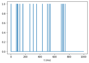
Aggregate spikes for all incoming neurons

N_in = 20

all_spikes = sum([spikes() for incoming_neuron in range(N_in)])

plot_signal(all_spikes);

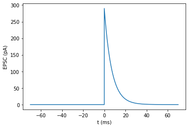
../_images/2020-07-06__Single_neuron_sim_19_0.png

EPSC’s¶

Simple step-and-exponential-decay impulse response.

Parameters estimated from fig. 5.14 in Dayan & Abott.

tau_EPSC = 7
height_EPSC = 290

T_support = 10*tau_EPSC
N_support = round(T_support/dt)
t_support = np.linspace(0, T_support, N_support)

EPSC = np.concatenate([
    np.zeros(N_support),
    np.exp(-t_support/tau_EPSC) * height_EPSC
])

plot_signal(EPSC, 'EPSC (pA)', t=np.concatenate([-t_support[::-1], t_support]));

../_images/2020-07-06__Single_neuron_sim_22_0.png

I = np.convolve(all_spikes, EPSC, mode='same')
plot_signal(I, 'I (pA)');

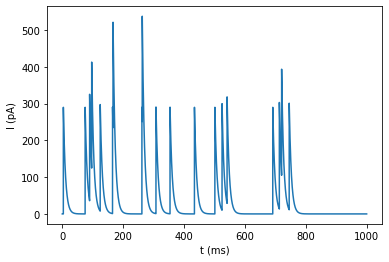
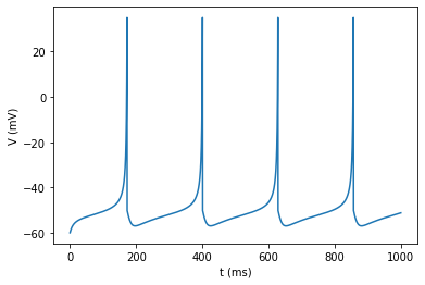
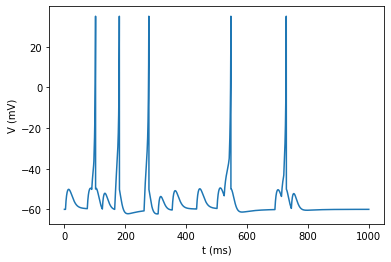
../_images/2020-07-06__Single_neuron_sim_23_0.png

Apply input to neuron¶

v = izh_neuron(I)
plot_signal(v, 'V (mV)');

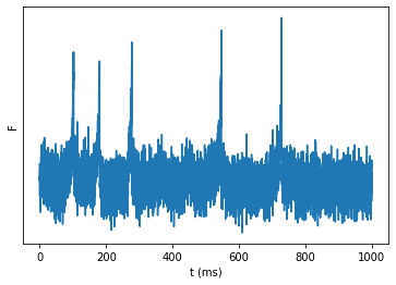
../_images/2020-07-06__Single_neuron_sim_25_0.png

Add voltage imaging noise¶

Gaussian noise, with \(\sigma\) from:

\(\text{SNR} = \frac{ΔV_{spike}}{\sigma_{noise}}\)

(see ‘Fidelity’ section from VI lit review).

SNR = 10
spike_height = v_peak - v_r

s_noise = spike_height / SNR
noise = np.random.randn(N)*s_noise
fig, ax = plot_signal(v+noise, 'F')
ax.set_yticks([]);

../_images/2020-07-06__Single_neuron_sim_27_0.png

Voltage-to-Wiring Sim

2020-07-06 • Single neuron simulation

Contents