Toggle navigation

.ipynb .pdf

repository open issue suggest edit

Binder

Contents

2022-08-21 • Area under STA (new conntest)

Imports

#

using Revise

using MyToolbox

using VoltoMapSim

[ Info: Precompiling VoltoMapSim [f713100b-c48c-421a-b480-5fcb4c589a9e]

Params

Based on Roxin; same as previous nb’s.

d = 6
p = get_params(
    duration = 10minutes,
    p_conn = 0.04,
    g_EE = 1   / d,
    g_EI = 18  / d,
    g_IE = 36  / d,
    g_II = 31  / d,
    ext_current = Normal(-0.5 * pA/√seconds, 5 * pA/√seconds),
    E_inh = -80 * mV,
    record_v = [1, 801],
);

Run sim

s = cached(sim, [p.sim]);

s = augment_simdata(s, p);

New connection test statistic

ii = s.input_info[1];

using PyPlot

[ Info: Precompiling Sciplotlib [61be95e5-9550-4d5f-a203-92a5acbc3116]

using VoltoMapSim.Plot

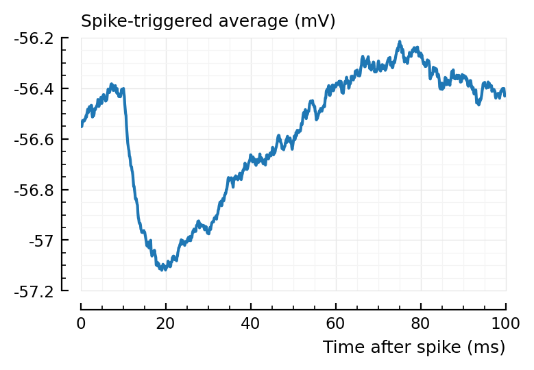
plotSTA(ii.v, ii.spiketrains.conn.inh[1], p);

sta = calc_STA(ii.v, ii.spiketrains.conn.inh[1], p);

t = sum(sta .- sta[1]);

What are the units? Sum of: voltage * dt.
So units are volt·second. But I’d had to add the dt to every term. I can do afterwards.

dt = p.sim.general.Δt;

t * dt / (mV * ms)

-3.55

(Estimate from graph for how big this should be: approx 0.5 mV difference, times 40 ms or so. So 20 mV·ms. Sure). How much is above and below?

sig = (sta .- sta[1]) * dt / (mV*ms)
above = sum(sig[sig .> 0])
below = sum(sig[sig .< 0])
above, below

(9, -12.5)

Nice, so yes units seem right.

How to name this measure. It’s area under STA, referenced to STA at t=0. AUS? AUA? relsum?
Area over start.
Just area is quite nice.

Adding this to misc.jl:

area(STA) = sum(STA .- STA[1]);

Compare performance

..between test measures: existing (peak-to-peak) and the new.

p0 = p;
pn = (@set p.conntest.STA_test_statistic = "area");

cached_conntest_perf = VoltoMapSim.cached_conntest_perf;

perf0 = cached_conntest_perf(1, ii.v, ii.spiketrains, p0);

perf0.detection_rates

(TPR_exc = 0.154, TPR_inh = 1, FPR = 0.15)

perfn = cached_conntest_perf(1, ii.v, ii.spiketrains, pn);

Testing connections: 100%|██████████████████████████████| Time: 0:00:24
Saving output at `C:\Users\tfiers\.phdcache\datamodel v2 (net)\evaluate_conntest_perf\51a268c55a44be7a.jld2` … done (4.5 s)

perfn.detection_rates

(TPR_exc = 0, TPR_inh = 0.8, FPR = 0.175)

Aha! It seems significantly worse than peak-to-peak (for this sim, this neuron).

Thing left to do is, use this to determine whether a presynaptic neuron is excitatory or inhibitory (now we’re cheating and presupposing that knowledge in the conntest perf eval).

I think it’s gonna make the performance way worse.

First, let’s redo the test for the inhibitory recorded neuron.

ii_inh = s.input_info[801];

perf0 = cached_conntest_perf(801, ii_inh.v, ii_inh.spiketrains, p0);

Testing connections: 100%|██████████████████████████████| Time: 0:00:20
Saving output at `C:\Users\tfiers\.phdcache\datamodel v2 (net)\evaluate_conntest_perf\6a503ee8521e347c.jld2` … done

perf0.detection_rates

(TPR_exc = 0.714, TPR_inh = 0.9, FPR = 0.05)

perfn = cached_conntest_perf(801, ii_inh.v, ii_inh.spiketrains, pn);

Testing connections: 100%|██████████████████████████████| Time: 0:00:21
Saving output at `C:\Users\tfiers\.phdcache\datamodel v2 (net)\evaluate_conntest_perf\352d0f0ba159fa0b.jld2` … done

perfn.detection_rates

(TPR_exc = 0.381, TPR_inh = 0.7, FPR = 0.1)

Again, signifcantly worse performance.

Use area for deciding exc or inh

This was the original motivation for this measure.

Our current test_connection returns a p-value based on peak-to-peak. It only says whether it thinks the presynaptic neuron is connected, not what type it is. We’ll add the area for that:

function test_connection_and_type(v, spikes, p)
    pval = test_connection(v, spikes, p)
    dt = p.sim.general.Δt
    A = area(calc_STA(v, spikes, p)) * dt / (mV*ms)
    if pval ≥ p.evaluation.α
        predicted_type = :unconn
    elseif A > 0
        predicted_type = :exc
    else
        predicted_type = :inh
    end
    return (; predicted_type, pval, area_over_start=A)
end;

test_connection_and_type(ii.v, ii.spiketrains.conn.inh[1], p)

(predicted_type = :inh, pval = 0.01, area_over_start = -3.55)

Performance optimization sidebar

@time test_connection_and_type(ii.v, ii.spiketrains.conn.inh[1], p)

  0.853824 seconds (1.35 k allocations: 22.599 MiB)

(predicted_type = :inh, pval = 0.01, area = -3.55)

Sidenote, shuffle connection test takes a while. Profiling shows that almost all time is spent in the calc_STA addition loop.

STA .+= @view VI_sig[a:b]

Doesn’t seem much more optimizable.

Wait, that broadcasting . is not necessary. Let’s see what perf is without.

@time test_connection_and_type(ii.v, ii.spiketrains.conn.inh[1], p)

  5.284591 seconds (720.96 k allocations: 5.469 GiB, 20.00% gc time)

(predicted_type = :inh, pval = 0.01, area = -3.55)

Huh, perf is worse with it, and way more allocations. Weird. Revert.

Trying with manual for loop (and @inbounds):

[..]

this made a type instability problem apparent (manual loop super slow. → @code_warntype. much red. problem was that Δt not inferred (cause simtype abstract). manually adding type made manual loop fast; and the prev, non manual loop also faster :))

Yes good, the new profile now also shows that the majority of time is spent in float:+, as it should be.

Now testing whether sim itself suffers from this same type instability problem..

# pshort = (@set p.sim.general.duration = 1*seconds);
# @code_warntype VoltoMapSim.init_sim(pshort.sim);
# state = VoltoMapSim.init_sim(pshort.sim);
#@code_warntype VoltoMapSim.step_sim!(state, pshort.sim, 1);

It doesn’t. Type known-ness (“stability”) seems good enough.

---

Back on topic

Now use the new test_connection_and_type in a reworked eval_conntest_perf function:

using DataFrames

# @cached key=[:m,:p] (
function evaluate_conntest_perf_v2(s, m, p)
    # s = augmented simdata
    # m = postsynaptic neuron ID
    @unpack N_tested_presyn, rngseed = p.evaluation;
    resetrng!(rngseed)
    function get_IDs_labels(IDs, label)
        N = min(length(IDs), N_tested_presyn)
        IDs_sample = sample(IDs, N, replace = false, ordered = true)
        return zip(IDs_sample, fill(label, N))
    end
    ii = s.input_info[m]
    IDs_labels = chain(
        get_IDs_labels(ii.exc_inputs, :exc),
        get_IDs_labels(ii.inh_inputs, :inh),
        get_IDs_labels(ii.unconnected_neurons, :unconn),
    )
    tested_neurons = DataFrame(
        input_neuron_ID = Int[],     # global ID
        real_type       = Symbol[],  # :unconn, :exc, :inh
        predicted_type  = Symbol[],  # idem
        pval            = Float64[],
        area_over_start = Float64[],
    )
    @showprogress (every = 400ms) "Testing connections: " (
    for (n, label) in collect(IDs_labels)  # `collect` necessary somehow
        test_result = test_connection_and_type(ii.v, s.spike_times[n], p)
        row = (input_neuron_ID = n, real_type = label, test_result...)
        push!(tested_neurons, Dict(pairs(row)))
    end)
    tn = tested_neurons
    det_rate(t) = count((tn.real_type .== t) .& (tn.predicted_type .== t)) / count(tn.real_type .== t)    
    detection_rates = (
        TPR_exc = det_rate(:exc),
        TPR_inh = det_rate(:inh),
        FPR = 1 - det_rate(:unconn),
    )
    return (; tested_neurons, detection_rates)
end
# end)

cached_eval(s, m, p) = cached(evaluate_conntest_perf_v2, [s, m, p], key = [m, p]);

Aside: @cached macro wish.
Also generates a $(funcname)_uncached. So here: evaluate_conntest_perf_uncached

# @profview evaluate_conntest_perf_v2(s, 1, p);

Testing connections: 100%|██████████████████████████████| Time: 0:00:32

^ Most time spent in the + and the setindex of the calc_STA loop. (A bit also in shuffle_ISIs). (Could speed up a bit maybe by having STA on the stack – prob using StaticArrays.jl – to save that setindex time. Though wouldn’t be major, as most time is still spent in float +). Another thing to try is @fastmath IEEE rules relaxing, to speed up the +.

testeval = cached_eval(s, 1, p);

Testing connections: 100%|██████████████████████████████| Time: 0:00:25
Saving output at `C:\Users\tfiers\.phdcache\datamodel v2 (net)\evaluate_conntest_perf_v2\b8c53748899be8e2.jld2` … done (6.9 s)

ENV["LINES"] = 100

100

testeval.detection_rates

(TPR_exc = 0, TPR_inh = 1, FPR = 0.125)

Comparison with before, when we didn’t predict the type (just connected or not) (from 2022-07-05__Network-conntest):

(TPR_exc = 0.154, TPR_inh = 1, FPR = 0.15)

The exc performance drops to zero. This is because all previously detected exc inputs are still detected, but classified as inhibitory, as seen in the below table.

The FPR rate is different because we now take a random sample of unconnected neurons to test (before, we took the first 40).

testeval.tested_neurons

76 rows × 5 columns

	input_neuron_ID	real_type	predicted_type	pval	area_over_start
	Int64	Symbol	Symbol	Float64	Float64
1	312	exc	unconn	0.51	11.3
2	565	exc	unconn	0.61	7.25
3	681	exc	unconn	0.55	6.58
4	597	exc	inh	0.02	-37.9
5	447	exc	unconn	0.68	1.42
6	766	exc	unconn	0.46	-7.55
7	132	exc	unconn	0.54	-20.9
8	139	exc	unconn	0.91	-22.8
9	446	exc	unconn	0.34	-27.5
10	194	exc	unconn	0.37	-31
11	710	exc	unconn	0.63	-38.1
12	352	exc	unconn	0.11	-19.9
13	11	exc	inh	0.01	-12.2
14	418	exc	inh	0.03	-21
15	101	exc	unconn	0.88	-1.2
16	629	exc	unconn	0.36	9.04
17	145	exc	unconn	0.47	-27.5
18	303	exc	unconn	0.05	-20
19	169	exc	unconn	0.68	1.38
20	66	exc	unconn	0.72	-21.2
21	70	exc	unconn	0.94	-0.564
22	800	exc	unconn	0.72	-39.6
23	516	exc	unconn	0.33	-28
24	136	exc	inh	0.02	-55.5
25	33	exc	unconn	0.86	-35.5
26	337	exc	unconn	0.56	-88.9
27	988	inh	inh	0.01	-3.55
28	894	inh	inh	0.01	-56.7
29	902	inh	inh	0.01	-59
30	928	inh	inh	0.01	-70.6
31	914	inh	inh	0.01	-52.1
32	831	inh	inh	0.01	-7.06
33	897	inh	inh	0.01	-72
34	829	inh	inh	0.01	-29.4
35	908	inh	inh	0.01	-63.8
36	922	inh	inh	0.01	-33.7
37	23	unconn	unconn	0.94	-4.49
38	25	unconn	unconn	0.75	14.4
39	86	unconn	unconn	0.11	-35.3
40	113	unconn	inh	0.03	-33.1
41	197	unconn	unconn	0.52	-11.8
42	227	unconn	unconn	0.84	-9.01
43	230	unconn	unconn	0.36	-1.34
44	262	unconn	unconn	0.45	-5.2
45	269	unconn	unconn	0.23	-32.9
46	323	unconn	unconn	0.08	-10.5
47	332	unconn	unconn	0.14	-15.5
48	367	unconn	unconn	0.96	-18.6
49	394	unconn	unconn	0.3	-10.7
50	410	unconn	unconn	0.37	1.49
51	424	unconn	unconn	0.12	-31.5
52	439	unconn	unconn	0.78	-39.4
53	460	unconn	unconn	0.17	-2.35
54	487	unconn	unconn	0.88	1.33
55	499	unconn	unconn	0.43	-13.4
56	521	unconn	unconn	0.85	1.62
57	537	unconn	unconn	0.14	-20.3
58	547	unconn	unconn	0.23	-35.3
59	599	unconn	inh	0.02	-48.4
60	612	unconn	unconn	0.22	-19.7
61	646	unconn	unconn	0.58	-0.319
62	669	unconn	unconn	0.73	-4.47
63	702	unconn	unconn	0.3	-26.1
64	722	unconn	unconn	0.11	-1.35
65	768	unconn	unconn	0.08	-10.7
66	790	unconn	unconn	0.18	-24.8
67	813	unconn	unconn	0.14	1.73
68	821	unconn	unconn	0.44	-0.367
69	842	unconn	exc	0.03	2.01
70	843	unconn	unconn	0.23	-10.6
71	875	unconn	inh	0.01	-7.61
72	882	unconn	unconn	0.18	-15.8
73	896	unconn	unconn	0.58	-19.3
74	921	unconn	exc	0.01	5.07
75	956	unconn	unconn	0.06	-18.9
76	977	unconn	unconn	0.49	-10.1

Inhibitory postsynaptic neuron

Now test input connections to the recorded inhibitory neuron:

te_inh = cached_eval(s, 801, p);

Testing connections: 100%|██████████████████████████████| Time: 0:00:21
Saving output at `C:\Users\tfiers\.phdcache\datamodel v2 (net)\evaluate_conntest_perf_v2\e828a750d5830742.jld2` … done

te_inh.detection_rates

(TPR_exc = 0.619, TPR_inh = 0.8, FPR = 0.075)

Comparison with before, as above:

(TPR_exc = 0.714, TPR_inh = 0.9, FPR = 0.05)

Results per neuron below. The area_over_start seems to work: exc is mostly positive (and thus predicted as exc), and vice versa for inhibitory/negative.

te_inh.tested_neurons

71 rows × 5 columns

	input_neuron_ID	real_type	predicted_type	pval	area_over_start
	Int64	Symbol	Symbol	Float64	Float64
1	544	exc	exc	0.01	156
2	345	exc	exc	0.01	41.6
3	468	exc	exc	0.01	74.1
4	206	exc	exc	0.01	147
5	689	exc	unconn	0.47	16.3
6	251	exc	exc	0.01	87.9
7	67	exc	exc	0.01	37.1
8	540	exc	exc	0.01	0.983
9	331	exc	exc	0.01	70.3
10	603	exc	exc	0.01	16.6
11	696	exc	unconn	0.07	31.2
12	693	exc	inh	0.04	-10.8
13	47	exc	unconn	0.37	54.6
14	533	exc	exc	0.01	190
15	513	exc	exc	0.01	89.5
16	639	exc	exc	0.01	68.5
17	615	exc	exc	0.01	37.6
18	55	exc	inh	0.01	-26.8
19	215	exc	unconn	0.06	65.5
20	411	exc	unconn	0.82	45.2
21	662	exc	unconn	0.12	-62.9
22	826	inh	unconn	0.63	-19.9
23	846	inh	exc	0.01	2.51
24	815	inh	inh	0.01	-31.6
25	937	inh	inh	0.01	-60.7
26	972	inh	inh	0.02	-10.4
27	857	inh	inh	0.01	-112
28	874	inh	inh	0.01	-43.1
29	981	inh	inh	0.01	-49.9
30	971	inh	inh	0.01	-26.3
31	896	inh	inh	0.01	-65.8
32	14	unconn	unconn	0.07	-21.8
33	65	unconn	unconn	0.22	70.9
34	76	unconn	unconn	0.92	19.3
35	172	unconn	unconn	0.05	18.3
36	179	unconn	unconn	0.56	-52.1
37	199	unconn	unconn	0.62	-39.1
38	201	unconn	unconn	0.5	-2.87
39	258	unconn	unconn	0.87	-47.2
40	283	unconn	unconn	0.11	29.7
41	357	unconn	inh	0.01	-7.26
42	385	unconn	inh	0.01	-38.2
43	387	unconn	unconn	0.94	-105
44	418	unconn	unconn	0.17	-42
45	424	unconn	unconn	0.96	-0.523
46	473	unconn	unconn	0.33	37.7
47	482	unconn	unconn	0.57	81.1
48	514	unconn	unconn	0.76	21.5
49	541	unconn	unconn	0.8	-37.1
50	556	unconn	unconn	0.21	9.93
51	568	unconn	unconn	0.81	-37.8
52	582	unconn	unconn	0.32	-19.5
53	600	unconn	unconn	0.16	-53.8
54	627	unconn	unconn	0.7	25.6
55	638	unconn	exc	0.01	29
56	659	unconn	unconn	0.66	-26.1
57	675	unconn	unconn	0.14	-83.3
58	684	unconn	unconn	0.65	-1.37
59	734	unconn	unconn	0.4	-88.9
60	746	unconn	unconn	0.89	5.16
61	777	unconn	unconn	0.55	105
62	798	unconn	unconn	0.14	14.4
63	830	unconn	unconn	0.24	-9.23
64	848	unconn	unconn	0.38	-1.16
65	889	unconn	unconn	0.79	-6.18
66	909	unconn	unconn	0.25	-18.2
67	927	unconn	unconn	0.08	-20.9
68	934	unconn	unconn	0.43	-30.4
69	952	unconn	unconn	0.45	-20.4
70	953	unconn	unconn	0.74	-25.5
71	964	unconn	unconn	0.25	-10.9

We missclassify an inhibitory input as excitatory because it’s “area over start” is positive. What does the STA look like?

plotSTA(s.signals[801].v, s.spike_times[846], p);

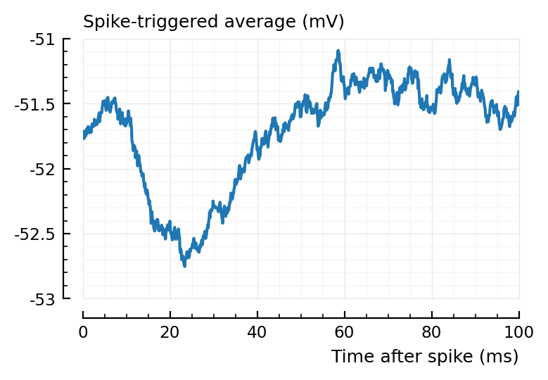
Looks nicely downwards..

area(calc_STA(s.signals[801].v, s.spike_times[846], p))

0.0251

But the area-over-start is indeed positive.

Could be remedied with a shorter STA window length.

For comparison, the STA of a correctly identified inh input:

plotSTA(s.signals[801].v, s.spike_times[815], p);

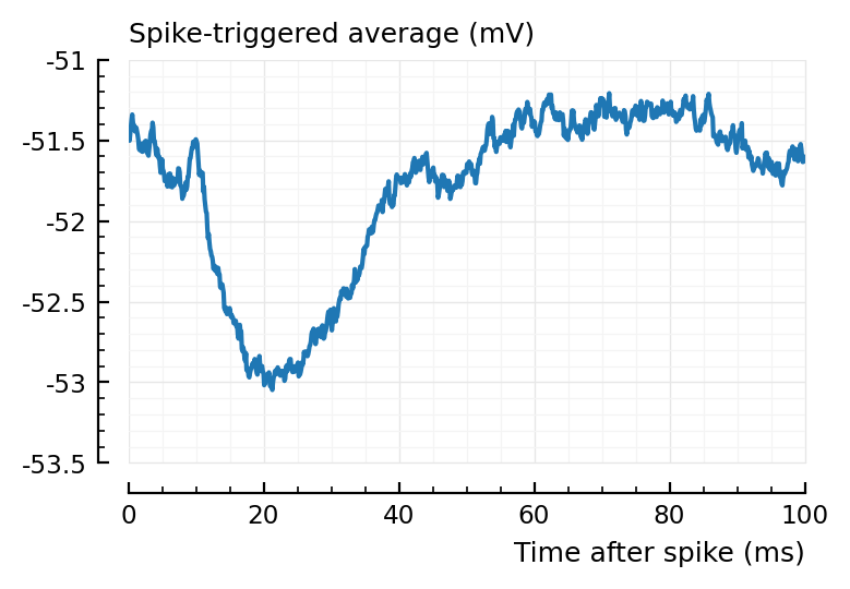
Looks very similar (the relative height of the positive and negative bumps).

The problem (the difference) is at t0.

---

Unrelated question (on previous results): Why are exc input STA’s on inh good, but on exc neurons so bad?

previous

2022-08-28 • Centred STAs

next

2022-08-17 • Investigate correlated spikers