Toggle navigation

.ipynb .pdf

repository open issue suggest edit

Binder

Contents

2023-02-07 • AdEx Nto1

(Based on 2023-01-19__[input], which is a distillation of 2022-10-24 • N-to-1 with lognormal inputs).

cd("/root/phd/pkg/SpikeWorks")
run(`git switch metdeklak`);

Your branch is up to date with 'origin/metdeklak'.

Already on 'metdeklak'

Imports

#

@showtime using Revise

using Revise: 0.599281 seconds (603.53 k allocations: 36.640 MiB, 3.70% gc time, 1.04% compilation time)

@showtime using MyToolbox
@showtime using SpikeWorks
@showtime using Sciplotlib
@showtime using VoltoMapSim

WARNING: using MyToolbox.@withfb in module Main conflicts with an existing identifier.
using MyToolbox: 1.574102 seconds (1.63 M allocations: 104.069 MiB, 2.92% gc time, 0.22% compilation time)
using SpikeWorks: 0.875073 seconds (1.28 M allocations: 78.734 MiB, 5.64% gc time)
using Sciplotlib: 9.385032 seconds (7.10 M allocations: 455.172 MiB, 2.42% gc time, 1.97% compilation time: 100% of which was recompilation)
using VoltoMapSim: 4.136105 seconds (4.98 M allocations: 328.876 MiB, 4.23% gc time)

AdEx equations & params

This is a distillation of previous notebook.

We base ourselves on

Richard Naud, Nicolas Marcille, Claudia Clopath, and Wulfram Gerstner,
‘Firing patterns in the adaptive exponential integrate-and-fire model’,
Biol Cybern, Nov. 2008, https://doi.org/10.1007/s00422-008-0264-7

..and their cortical RS (regular spiking) neuron in table 1.

Param value comparison, for cortical RS neuron

(Table repeted from prev notebook)

Naud 2008 AdEx	Val	Val	Izh / report	What
\(C\)	104 pF	100 pF	\(C\)
\(C/g_L\)	24 ms	?	?	Time constant of voltage
		0.14 ms·mV	\(C/k\)	?
————–	———	————	————–
\(g_L\)	4.3 nS	14 nS	\(k(v_t-v_r)\)	Slope of V̇(V) at rest
\(E_L\)	-65 mV	-60 mV	\(v_r\)	Rest (stable fixed point)
\(V_T\)	-52 mV	-50 mV	\((v_t+v_r)/2\)	Minimum of V̇(V)
	-49.6 mV	-40 mV	\(v_t\)	Threshold (unstable fixed point)
	82 nS	14 nS	\(k(v_t-v_r)\)	Slope of V̇(V) at threshold
\(Δ_T\)	0.8 mV
————–	———	————	————–
\(a\)	-0.8 nS	-2 nS	\(b\)	Sensitivity of adapt. current
\(τ_w\)	88 ms	33 ms	\(a^{-1}\)	Time ct of adapt. current
\(b\)	65 pA	100 pA	\(d\)	Adapt. current bump after spike
\(V_r\)	-53 mV	-50 mV	\(c\)	Reset voltage after spike

Start of code

@typed begin
    # AdEx LIF neuron params (cortical RS)
    C  = 104  * pF
    gₗ = 4.3  * nS
    Eₗ = -65  * mV
    Vₜ = -52  * mV
    Δₜ = 0.8  * mV 
    Vₛ =   0  * mV
    Vᵣ = -53  * mV
    a  = 0.8  * nS
    b  =  65  * pA
    τw =  88  * ms 
    # Conductance-based synapses
    Eₑ =   0 * mV
    Eᵢ = -80 * mV
    τ  =   7 * ms
end;

Simulated variables and their initial values

x₀ = (
    # AdEx variables
    v   = Vᵣ,      # Membrane potential
    w   = 0 * pA,  # Adaptation current
    # Synaptic conductances g
    gₑ  = 0 * nS,  # = Sum over all exc. synapses
    gᵢ  = 0 * nS,  # = Sum over all inh. synapses
);

\[\begin{split} \begin{align} C \frac{dV}{dt} &= -g_L (V - E_L) + g_L \Delta_T \exp \left( \frac{V - V_T}{\Delta_T} \right) + I - w\\ \tau_w \frac{dw}{dt} &= a (V - E_L) - w \end{align} \end{split}\]

if \(V > 0\) mV, then

\[\begin{split} \begin{align} V &→ V_r\\ w &→ w + b \end{align} \end{split}\]

Differential equations:

calculate time derivatives of simulated vars
(and store them “in-place”, in Dₜ).

function f!(Dₜ, vars)
    v, w, gₑ, gᵢ = vars

    # Conductance-based synaptic current
    Iₛ = gₑ*(v-Eₑ) + gᵢ*(v-Eᵢ)

    # AdEx 2D system
    Dₜ.v = (-gₗ*(v-Eₗ) + gₗ*Δₜ*exp((v-Vₜ)/Δₜ) - Iₛ - w) / C
    Dₜ.w = (a*(v-Eₗ) - w) / τw

    # Synaptic conductance decay
    Dₜ.gₑ = -gₑ / τ
    Dₜ.gᵢ = -gᵢ / τ
end;

We correct the sign of Iₛ.
From prev nb:

Positive charges flowing out of membrane: Iₘₑₘ pos.
Positive charges flowing from electrode into cell: Iₑₓₜ pos.

v is usually < Eₑ,
so (v-Eₑ) will be negative.
But it should be positive, if we want to have + Iₛ in our Dₜ.v equation.

Eh no, I’ll keep as is.
Consistency with Iₘₑₘ (but against convention, yes).

Spike discontinuity

has_spiked(vars) = (vars.v > Vₛ)

function on_self_spike!(vars)
    vars.v = Vᵣ
    vars.w += b
end;

Conductance-based AdEx neuron

coba_adex_neuron = NeuronModel(x₀, f!; has_spiked, on_self_spike!);

---

The rest (i.e. the Nto1 part, with E:I) is same

More parameters, and input spikers

using SpikeWorks.Units
using SpikeWorks: LogNormal

@typed begin
    Δt = 0.1ms
    sim_duration = 10minutes
end

600

Firing rates λ for the Poisson inputs

fr_distr = LogNormal(median = 4Hz, g = 2)

Distributions.LogNormal{Float64}(μ=1.39, σ=0.693)

@enum NeuronType exc inh

input(;
    N = 100,
    EIratio = 4//1,
    scaling = N,
) = begin
    firing_rates = rand(fr_distr, N)
    input_IDs = 1:N
    inputs = [
        Nto1Input(ID, poisson_SpikeTrain(λ, sim_duration))
        for (ID, λ) in zip(input_IDs, firing_rates)
    ]
    # Nₑ, Nᵢ = groupsizes(EIMix(N, EIratio))
    EImix = EIMix(N, EIratio)
    Nₑ = EImix.Nₑ
    Nᵢ = EImix.Nᵢ
    neuron_type(ID) = (ID ≤ Nₑ) ? exc : inh
    Δgₑ = 60nS / scaling
    Δgᵢ = 60nS / scaling * EIratio
    on_spike_arrival!(vars, spike) =
        if neuron_type(source(spike)) == exc
            vars.gₑ += Δgₑ
        else
            vars.gᵢ += Δgᵢ
        end
    return (;
        firing_rates,
        inputs,
        on_spike_arrival!,
        Nₑ,
    )
end;

using SpikeWorks: Simulation, step!, run!, unpack, newsim,
                  get_new_spikes!, next_spike, index_of_next

new(; kw...) = begin
    ip = input(; kw...)
    s = newsim(coba_adex_neuron, ip.inputs, ip.on_spike_arrival!, Δt)
    (sim=s, input=ip)
end;

Multi sim

(These Ns are same as in e.g. https://tfiers.github.io/phd/nb/2022-10-11__Nto1_output_rate__Edit_of_2022-05-02.html)

using SpikeWorks: spikerate

sim_duration/minutes

10

using Printf
print_Δt(t0) = @printf("%.2G seconds\n", time()-t0)
macro timeh(ex) :( t0=time(); $(esc(ex)); print_Δt(t0) ) end;

Ns_and_scalings = [
    (5,    2.4),   # => N_inh = 1
    (20,   1.3),
        # orig: 21.
        # But: "pₑ = 0.8 does not divide N = 21 into integer parts"
        # So voila
    (100,  0.8),
    (400,  0.6),
    (1600, 0.5),
    (6500, 0.5),
];
Ns = first.(Ns_and_scalings);

nbname = "2023-02-07__AdEx_Nto1"
cachekey(N) = "$(nbname)__N=$(N)__T=$(sim_duration)";
cachekey(Ns[end])

"2023-02-07__AdEx_Nto1__N=6500__T=600"

function runsim(N, scaling)
    println()
    (sim, inp) = new(; N, scaling)
    @show N
    @timeh run!(sim)
    @show spikerate(sim)
    return (; sim, input=inp)
end 

simruns = []
for (N, f) in Ns_and_scalings
    scaling = f*N
    simrun = cached(runsim, (N, scaling), key=cachekey(N))
    push!(simruns, simrun)
end

Loading cached output from `/root/.phdcache/runsim/2023-02-07__AdEx_Nto1__N=5__T=600.jld2` … done (5.4 s)
Loading cached output from `/root/.phdcache/runsim/2023-02-07__AdEx_Nto1__N=20__T=600.jld2` … done (0.1 s)
Loading cached output from `/root/.phdcache/runsim/2023-02-07__AdEx_Nto1__N=100__T=600.jld2` … done (0.1 s)
Loading cached output from `/root/.phdcache/runsim/2023-02-07__AdEx_Nto1__N=400__T=600.jld2` … done (0.1 s)
Loading cached output from `/root/.phdcache/runsim/2023-02-07__AdEx_Nto1__N=1600__T=600.jld2` … done (0.3 s)
Loading cached output from `/root/.phdcache/runsim/2023-02-07__AdEx_Nto1__N=6500__T=600.jld2` … done (0.8 s)

sims = first.(simruns)
inps = last.(simruns);

Base.summarysize(simruns[6]) / GB

0.523

Disentangle

spiketimes(input::Nto1Input) = input.train.spiketimes;

vrec(s::Simulation{<:Nto1System}) = s.rec.v;

---

/ end same

Plot

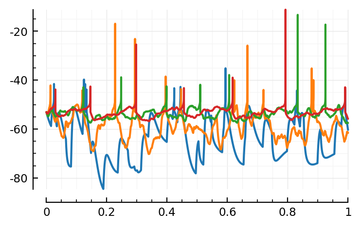
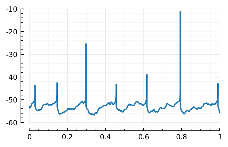
Let’s see what this AdEx guy looks like.

plot1(i) = begin
    s = sims[i]
    Nt = s.stepcounter.N
    t = linspace(0, sim_duration, Nt)
    plotsig(t, vrec(s) / mV; tlim=[0, 1seconds])
end
plot1(1)
plot1(3)
plot1(5)
plot1(6);

plot1(6);

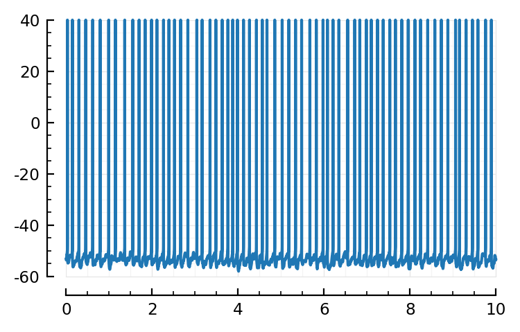
Now to recreate the plot of https://tfiers.github.io/phd/nb/2022-10-24__Nto1_with_fixed_lognormal_inputs.html#plot

We’ll add fake spikes up to our previous’ spike cutoff.

i = 6
s = sims[i]
v = copy(s.rec.v);
v[to_timesteps.(s.rec.spiketimes, Δt)] .= 40mV
Nt = s.stepcounter.N
t = linspace(0, sim_duration, Nt)
plotsig(t, v / mV; tlim=[0, 10seconds]);

Conntest pooled windows - linear regress 10 ms

i = 6
N = Ns[i]

6500

inp = inps[i];

Nₑ = inp.Nₑ

5200

include("/root/phd/nb/2023-02-07__[input-linefit-wins].jl");

wins = windows(6, 1);
X, y = build_Xy(wins);

ts = @view X[:,2]
sel = 1:10000

Sciplotlib.plot(ts[sel]*Δt/ms, y[sel]/mV, ".", alpha=0.1);

So we still see our ramp-ups; but much less so.
(compare, https://tfiers.github.io/phd/nb/2023-01-19__Fit-a-line.html#plot-some-windows)

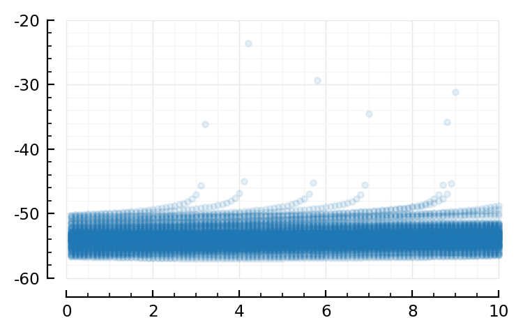
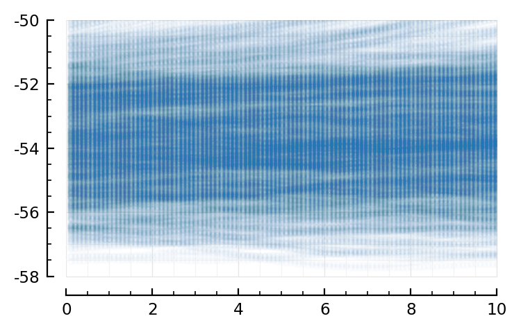
Now the zoom-in

Ny = length(y)

280500

(only 0.3M datapoints here; but in the other nb we used our highest-firing).

sel = 1:100_000
Sciplotlib.plot(
    ts[sel]*Δt/ms,
    y[sel]/mV,
    ".";
    alpha = 0.01,
    ylim = [-58, -50],  # mV
    clip_on = true,
);

inh_neurons = Nₑ+1:N;

spiketimes(i::Int) = spiketimes(inp.inputs[i]);

shuffle_sources = sample(1:N, 100, replace=true)

real_spiketrains = spiketimes.(1:N);
unconnected_trains = shuffle_ISIs.(spiketimes.(shuffle_sources));

all_spiketrains = [real_spiketrains; unconnected_trains];

using Base.Threads: @threads

Nrows = length(all_spiketrains)

6600

(Below calc takes 3’25 on laptop, 7 threads)

makerows() = begin
    rows = Vector(undef, Nrows)
    p = Progress(Nrows)
    @threads for r in 1:Nrows
        rows[r] = makerow(r)
        next!(p)
    end
    return rows
end;

rows = cached(makerows, (), key=cachekey(N));

Loading cached output from `/root/.phdcache/makerows/2023-02-07__AdEx_Nto1__N=6500__T=600.jld2` … done (0.1 s)

df = DataFrame(rows)
disp(df, 5)  # (huh, disp no work no more here)

6600×4 DataFrame

6575 rows omitted

Row	conntype	slope	pval	predtype
	Symbol	Float64	Float64	Symbol
1	exc	-0.28	0.813	unconn
2	exc	0.828	0.584	unconn
3	exc	3.78	1.44E-05	exc
4	exc	5.42	0.00335	unconn
5	exc	1.85	0.0458	unconn
6	exc	4.7	9.53E-05	exc
7	exc	-1.3	0.26	unconn
8	exc	8.08	0.000785	exc
9	exc	1.65	0.00208	unconn
10	exc	8.21	6.55E-05	exc
11	exc	4.46	0.00175	unconn
12	exc	3.78	0.000389	exc
13	exc	2.73	0.00868	unconn
⋮	⋮	⋮	⋮	⋮
6589	unconn	3.52	0.0157	unconn
6590	unconn	0.62	0.428	unconn
6591	unconn	0.275	0.818	unconn
6592	unconn	-0.95	0.391	unconn
6593	unconn	-0.67	0.118	unconn
6594	unconn	4.07	0.002	unconn
6595	unconn	0.0647	0.961	unconn
6596	unconn	2.65	0.171	unconn
6597	unconn	-4.21	9.3E-06	inh
6598	unconn	-1.86	0.221	unconn
6599	unconn	0.427	0.612	unconn
6600	unconn	-2.7	0.0612	unconn

perftable(df)

Tested connections: 6600
		┌───────	Real type	───────┐		Precision
		unconn	exc	inh
┌	unconn	86	3712	730		2%
Predicted type	exc	11	1326	10		98%
└	inh	3	161	561		77%
Sensitivity		86%	26%	43%

At this arbitrary ‘α’ = 0.001:

• FPR: 14%

• TPRₑ: 26%

• TPRᵢ: 43%

Comparing with the results with the Izh neuron:
(https://tfiers.github.io/phd/nb/2023-01-19__Fit-a-line.html#proper-eval)\

• FPR: 34%

• TPRₑ: 24%

• TPRᵢ: 37%

So, that seems like a def increase :)

Now with lower FPR / lower α

Nrows = length(all_spiketrains)
# Nrows = 20

6600

α=0.0001;
rows2 = Vector(undef, Nrows)
p = Progress(Nrows)
@threads for r in 1:Nrows
    rows2[r] = makerow(r; α)
    next!(p)
end;
df2 = DataFrame(rows2)
perftable(df2)

Progress: 100%|█████████████████████████████████████████| Time: 0:04:54Progress:  73%|█████████████████████████████▊           |  ETA: 0:01:21

Tested connections: 6600
		┌───────	Real type	───────┐		Precision
		unconn	exc	inh
┌	unconn	84	4143	857		2%
Predicted type	exc	3	965	2		99%
└	inh	13	91	442		81%
Sensitivity		84%	19%	34%

(FPR 16%)

Even lowerr

It’s dumb to recalculate; we have the p-values.

(Plus, there’s some memory thing it seems: process dies halfway here).

update_predtype(row::DataFrameRow; α) = begin
    if row.pval < α
        predtype = (row.slope > 0 ? :exc : :inh)
    else
        predtype = :unconn
    end
    row.predtype = predtype
end;

df3 = deepcopy(df)
foreach(row -> update_predtype(row, α = 0.0000008), eachrow(df3))
perftable(df3)

Tested connections: 6600
		┌───────	Real type	───────┐		Precision
		unconn	exc	inh
┌	unconn	95	4666	1019		2%
Predicted type	exc	5	501	1		99%
└	inh	0	32	281		90%
Sensitivity		95%	10%	22%

:D

Conntest STA

winsize = 1000

calcSTA(sim, spiketimes) =
    calc_STA(vrec(sim), spiketimes, sim.Δt, winsize);

# @code_warntype calc_STA(vrec(s), st1, s.Δt, winsize)
# all good

Cache STA calc

using Base.Threads: @threads

function calc_STA_and_shufs(spiketimes, sim)
    realSTA = calcSTA(sim, spiketimes)
    shufs = [
        calcSTA(sim, shuffle_ISIs(spiketimes))
        for _ in 1:100
    ]
    (; realSTA, shufs)
end

"calc_all_STAs_and_shufs"
function calc_all_STAz(inputs, sim)
    f(input) = calc_STA_and_shufs(spiketimes(input), sim)
    N = length(inputs)
    res = Vector(undef, N)
    p = Progress(N)
    # @threads for i in 1:N
    for i in 1:N
        res[i] = f(inputs[i])
        next!(p)
    end
    res
end
calc_all_STAz(simrun) = calc_all_STAz(unpakk(simrun)...);
unpakk(simrun) = (; simrun.input.inputs, simrun.sim);

# out = calc_all_STAz(simruns[1])
# print(Base.summary(out))

calc_all_cached(i) = cached(calc_all_STAz, [simruns[i]], key=cachekey(Ns[i]))

out = []
for i in eachindex(simruns)
    push!(out, calc_all_cached(i))
end;

Loading cached output from `/root/.phdcache/calc_all_STAz/2023-02-07__AdEx_Nto1__N=5__T=600.jld2` … done (0.3 s)
Loading cached output from `/root/.phdcache/calc_all_STAz/2023-02-07__AdEx_Nto1__N=20__T=600.jld2` … done
Loading cached output from `/root/.phdcache/calc_all_STAz/2023-02-07__AdEx_Nto1__N=100__T=600.jld2` … done (0.2 s)
Loading cached output from `/root/.phdcache/calc_all_STAz/2023-02-07__AdEx_Nto1__N=400__T=600.jld2` … done (1.0 s)
Loading cached output from `/root/.phdcache/calc_all_STAz/2023-02-07__AdEx_Nto1__N=1600__T=600.jld2` … done (4.8 s)
Progress:  55%|██████████████████████▍                  |  ETA: 0:15:39

conntype_vec(i) = begin
    sim, inp = simruns[i]
    Nₑ = inp.Nₑ
    N = Ns[i]
    conntype = Vector{Symbol}(undef, N);
    conntype[1:Nₑ]     .= :exc
    conntype[Nₑ+1:end] .= :inh
    conntype
end;

conntestresults(i, teststat = ptp_test; α = 0.05) = begin
    
    f((sta, shufs)) = test_conn(teststat, sta, shufs; α)
    res = @showprogress map(f, out[i])
    df = DataFrame(res)
    df[!, :conntype] = conntype_vec(i)
    df
end;

# conntestresults(1)

using Sciplotlib: plot

spikerate_(spiketimes) = length(spiketimes) / sim_duration;

spikerate_(inp::Nto1Input) = spikerate_(spiketimes(inp));

firing_rates(i) = spikerate_.(spiketimes.(inps[i].inputs));

previous

2023-04-11 • Nto1 AdEx sims: conntest method comparison

next

2023-02-07 • [input] to ‘AdEx Nto1’