Toggle navigation

.ipynb .pdf

repository open issue suggest edit

Binder

Contents

2022-07-01 • g_EI

Playing with the between-group synaptic strengths and their effect on firing rate distributions.

Imports

#

using Revise

using MyToolbox

using VoltoMapSim

[ Info: Precompiling VoltoMapSim [f713100b-c48c-421a-b480-5fcb4c589a9e]

Sim

import PyPlot

using VoltoMapSim.Plot

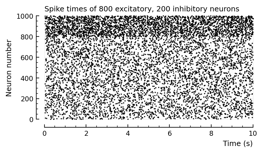
function sim_and_plot(; params...)
    p = get_params(; params...)
    s = cached(sim, [p.sim])
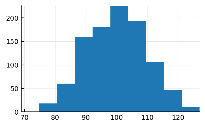
    num_spikes = length.(s.spike_times)
    sum(num_spikes) > 0 || error("no spikes")
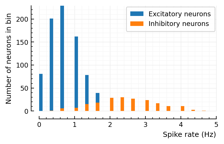
    spike_rates = num_spikes ./ p.sim.general.duration
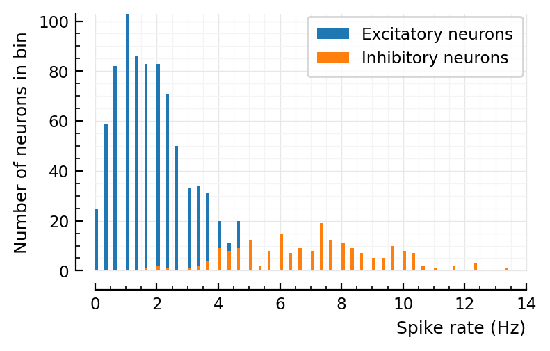
    histplot_fr(spike_rates)
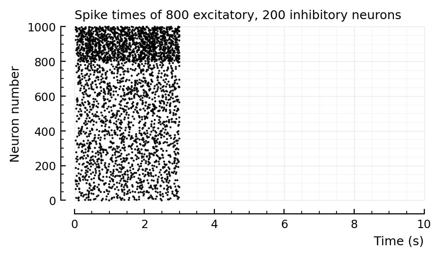
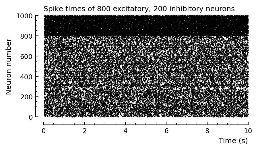
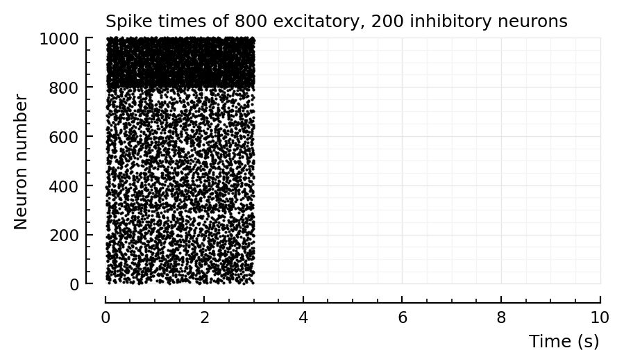
    rasterplot(s.spike_times, tlim=[0,10]seconds)
    return p, s, spike_rates
end;

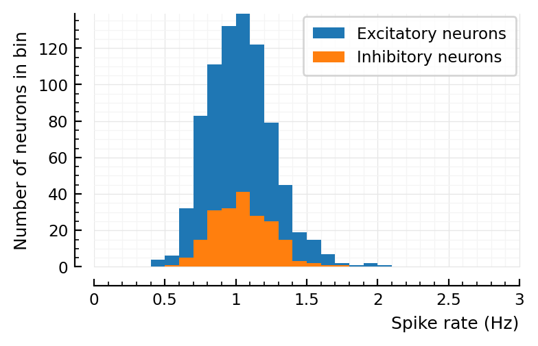
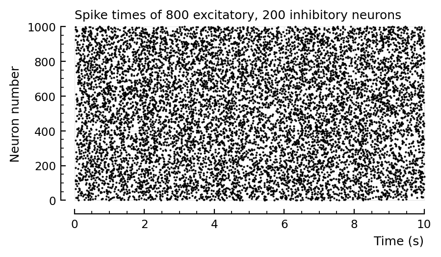
4:1

sim_and_plot(
    duration = 20seconds,
    g_EE = 1,
    g_EI = 1,
    g_IE = 4,
    g_II = 4,
);
# Default values

d = 2  # to lower firing rate
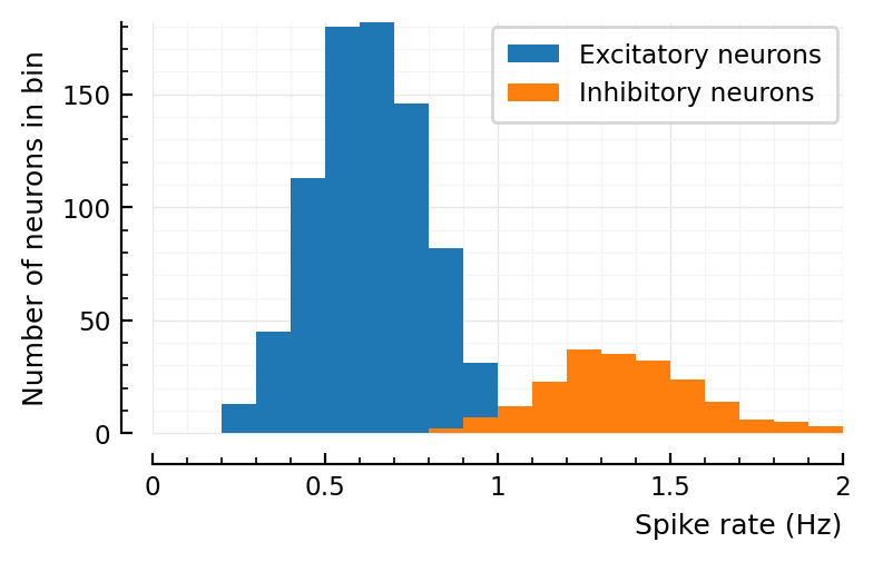
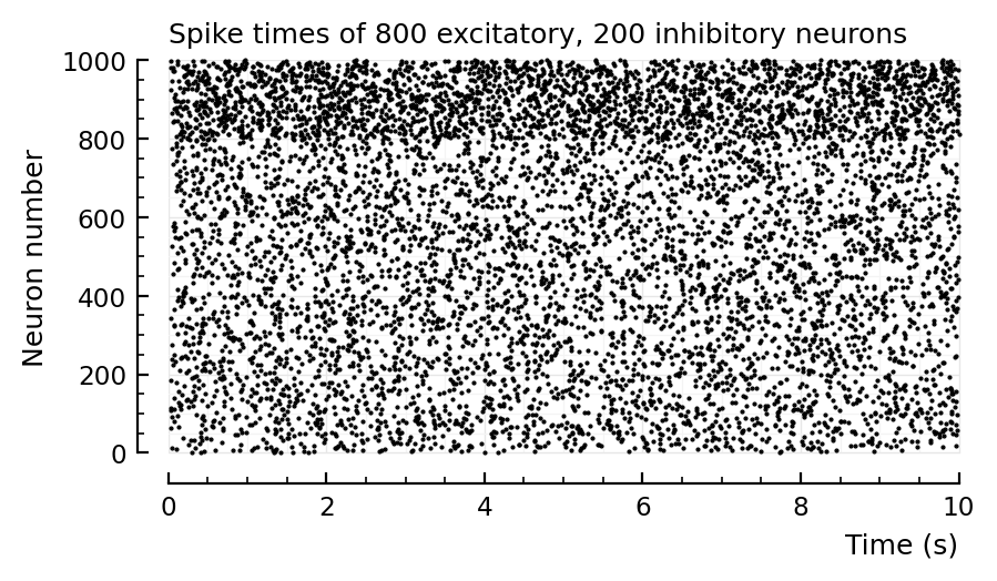
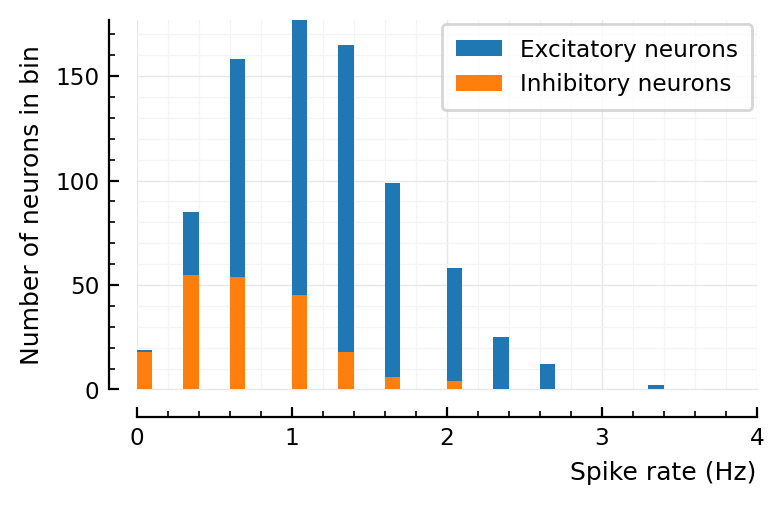
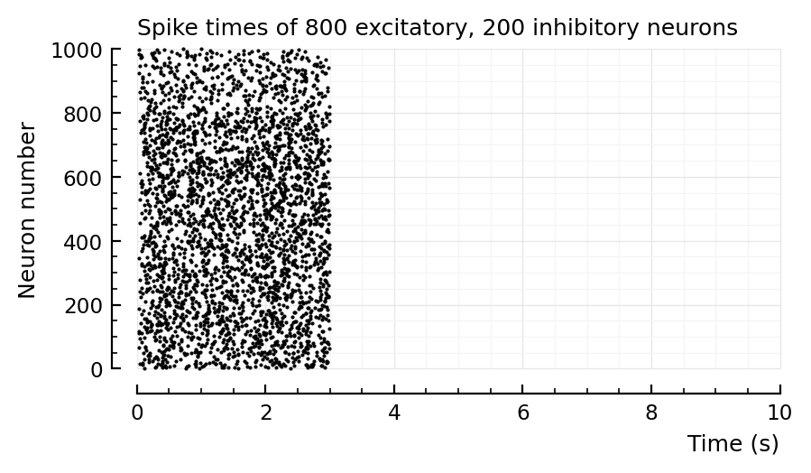
sim_and_plot(
    duration = 20seconds,
    g_EE = 1 / d,
    g_EI = 4 / d,
    g_IE = 1 / d,
    g_II = 4 / d,
);
# Previous, wrong values

Aggregated over E and I, you can indeed be fooled that the fr histogram is lognormal.

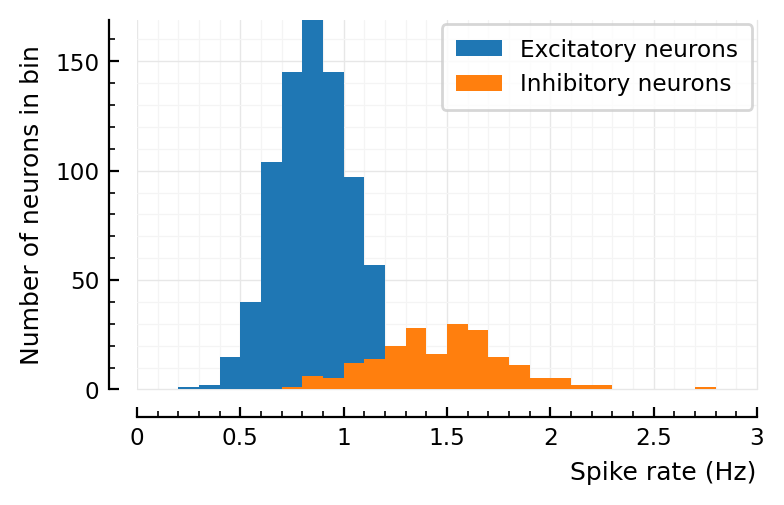
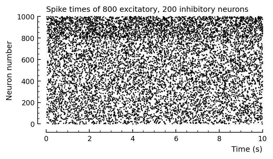
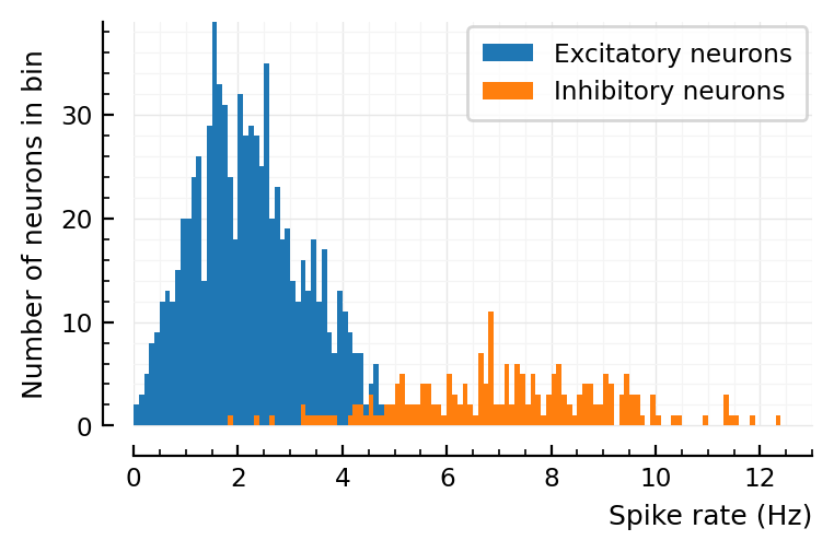
Roxin2011

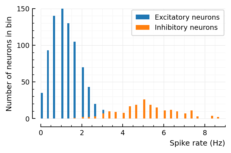
d = 6
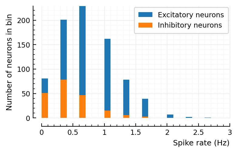
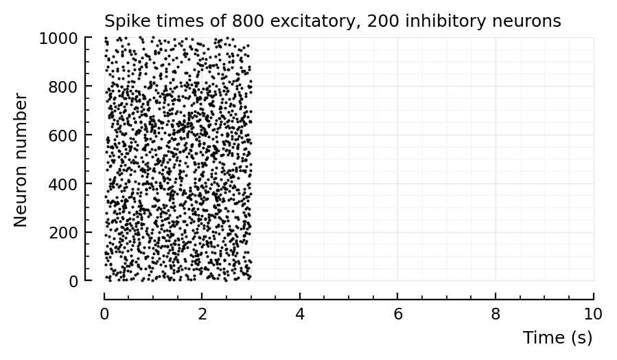
p, s, spike_rates = sim_and_plot(
    duration = 10seconds,
    g_EE = 1   / d,
    g_EI = 18  / d,
    g_IE = 36  / d,
    g_II = 31  / d,
);
# Roxin2011 values

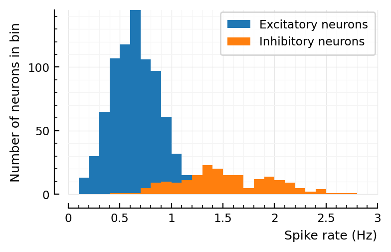
Recreating plots from roxin.
Here: aggregate spike rates of inh and exc, on log scale

bins = exp10.(-1:0.2:1)
fig, ax = plt.subplots()
ax.hist(spike_rates; bins, histtype="step")
set(ax, xscale="log", xlabel="Firing rate (Hz)", xlim=(0.1,10));

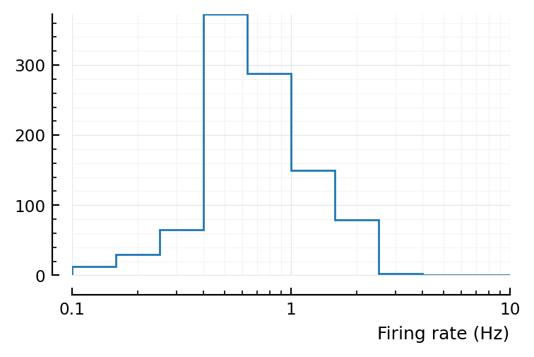
Note that Roxin firing rates have much wider range: from 0.01 to 100

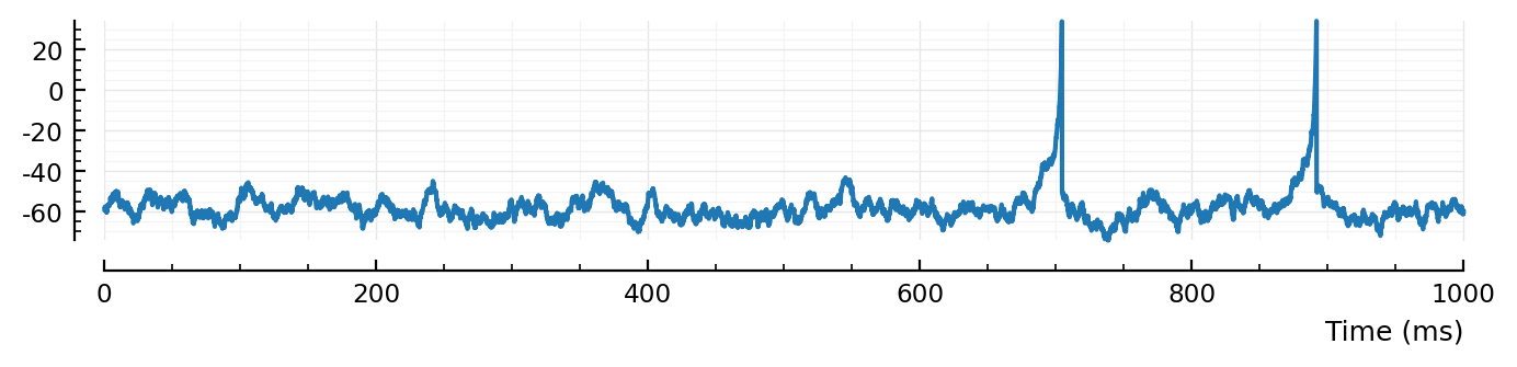
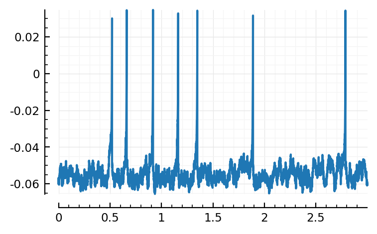
fig, ax = plt.subplots(figsize=(8,1.3))
plotsig(s.timesteps / ms, s.voltage_traces[1] / mV; ax, tlim=[0,1000], xlabel="Time (ms)");

No lognormal weights

Roxin2011 finds that wider synaptic strength distribution gives narrower firing rate distribution. So let’s do as they do in most plots, and give no variance at all to the synaptic weights.

d = 6
p, s, spike_rates = sim_and_plot(
    duration = 20seconds,
    g_EE = 1   / d,
    g_EI = 18  / d,
    g_IE = 36  / d,
    g_II = 31  / d,
    syn_strengths = LogNormal_with_mean(20nS, 0)  # ← zero variance
);
# Roxin2011 values

Running simulation: 100%|███████████████████████████████| Time: 0:00:09
Saving output at `C:\Users\tfiers\.phdcache\datamodel v2 (net)\sim\61e108c7773a503f.jld2` … done (0.2 s)

Result: nope. Not wider

Positive-mean input current

Positive as in: excitatory. (Previous defaults had zero-mean input current. But Roxin had positive mean; dV/dt ~ +I_ext in their eq. In our eq, dV/dt ~ –I_ext).

Also, they have lower p_conn than our default of 10%. (Result after changing this: not much difference)

1/√.1ms

3162.277660168379

d = 6
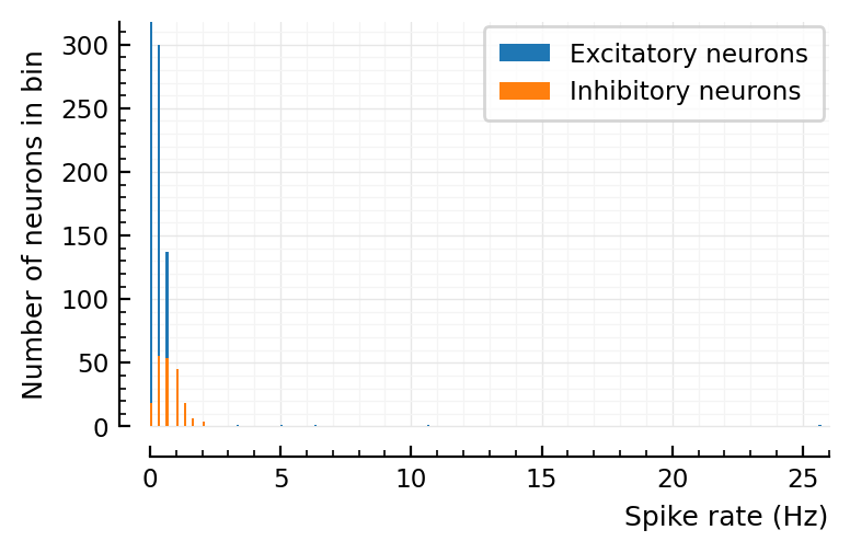
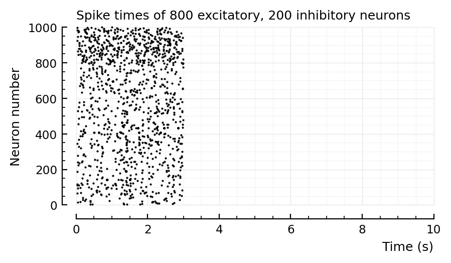
p, s, spike_rates = sim_and_plot(
    duration = 3seconds,
    p_conn = 0.04,
    g_EE = 1   / d,
    g_EI = 18  / d,
    g_IE = 36  / d,
    g_II = 31  / d,
    ext_current = Normal(-0.42 * pA/√seconds, 4 * pA/√seconds),
);
# Roxin2011 values

Running simulation: 100%|███████████████████████████████| Time: 0:00:01
Saving output at `C:\Users\tfiers\.phdcache\datamodel v2 (net)\sim\2d8e1e3dedc55948.jld2` … done (0.1 s)

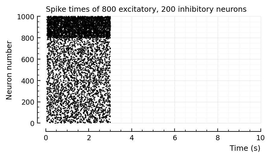
The longer you simulate, the narrower both distributions seem to become.

So I could see obtaining the approximate results of Roxin2011 figure 8:

• simulate for a short time (they did not report their simulation time. But given that they have 2000x the number of neurons as us here, it can’t have been very long).

• give the inhibitory neurons less external current (which is indeed what they did): their distribution will then overlap more with the excitatory one

• plot the firing rates in aggregate (not separate as I did here).

Shape of normal on log scale

x = 1:0.01:10
y = @. exp(-(x-5)^2 / 3)
fig,ax = plt.subplots()
ax.plot(x,y);
set(ax, xscale="log");

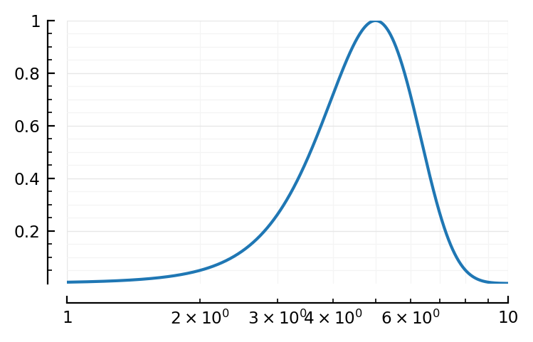
Looks like the “very close to lognormal” plots in roxin.

Truncated normal is ‘heavy tailed’

Fig 5C of Roxin

distr = TruncatedNormal(1Hz, 7Hz, 0Hz, Inf*Hz)  # mean, std, left bound, right bound
fr = rand(distr, 12500)
plt.hist(fr, bins=30, ec="k", fc="w")
plt.plot(mean(fr), -50, "w^", clip_on=false, mec="k", ms=8)
plt.plot(median(fr), -50, "k^", clip_on=false, mec="k", ms=8)
plt.ylim(bottom=0)
plt.xlim(0, 40);

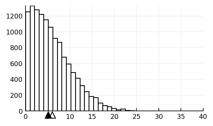
median(fr), mean(fr)

(5.1193548485998175, 5.988978579872706)

tbf Roxin had a bit larger diff between these.

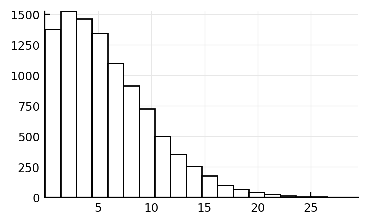
Sum of two normals

distr = truncated(MixtureModel(Normal, [(2Hz,5Hz), (8Hz,6Hz)], [0.8, 0.2]), lower=0Hz)
fr = rand(distr, 10_000)
plt.hist(fr, bins=20, ec="k", fc="w");

log scale:

bins = exp10.(-1:0.2:3)
fig, ax = plt.subplots()
ax.hist(fr; bins, histtype="step")
set(ax, xscale="log", xlim=(0.1,100));

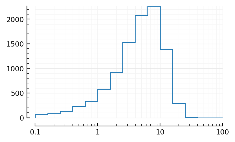
Looks very much like fig 8D.

Sanity check

p, s, spike_rates = sim_and_plot(
    duration = 3seconds,
    g_EE = 0,
    g_EI = 0,
    g_IE = 600,
    g_II = 0,
    to_record = [696],
);

Running simulation: 100%|███████████████████████████████| Time: 0:00:01
Saving output at `C:\Users\tfiers\.phdcache\datamodel v2 (net)\sim\4154eaf3081de0da.jld2` … done (0.8 s)

s.spike_times[812] / ms .+ 10

1-element Vector{Float64}:
 1021.599999999905

s.spike_times[696] / ms

10-element Vector{Float64}:
 1022.0999999999038
 1022.2999999999038
 1022.4999999999038
 1022.8999999999038
 1023.2999999999037
 1023.6999999999036
 1024.0999999999037
 1024.4999999999036
 1025.0999999999035
 1025.8999999999035

v,u,g_exc,g_inh = s.signals[696];

@unpack E_exc, E_inh = p.sim.general.synapses
I = @. (  g_exc * (v - E_exc)
        + g_inh * (v - E_inh));

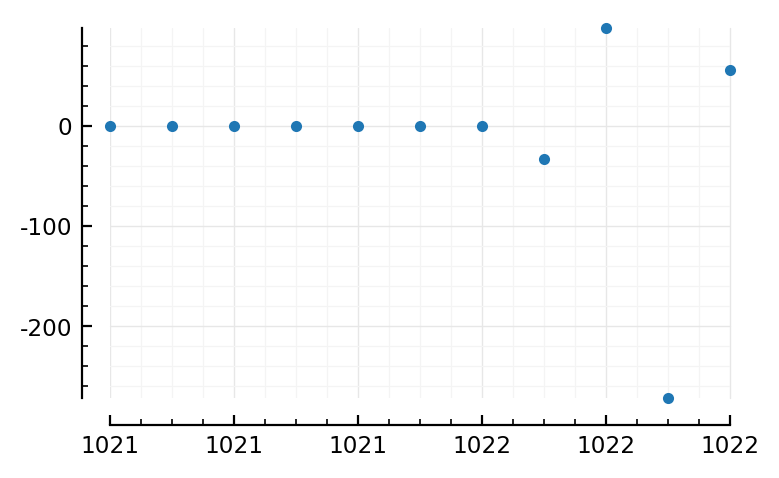
plotsig(s.timesteps / ms, (v .- E_inh) / mV, tlim=[1021,1022], marker=".", linestyle="None");

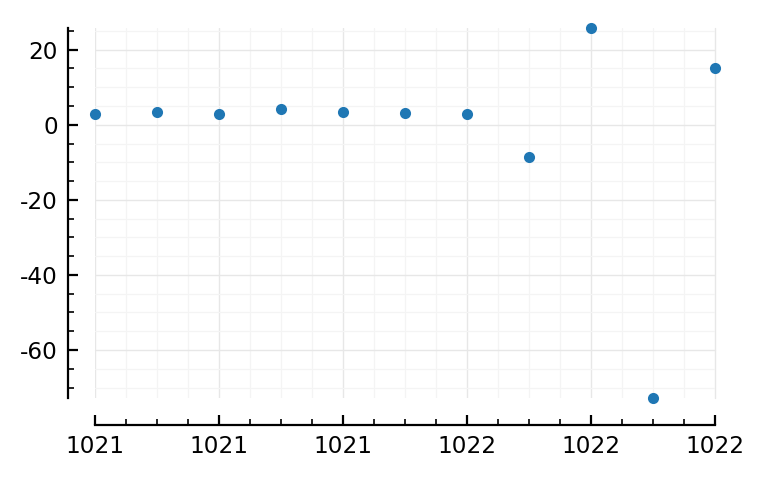
plotsig(s.timesteps / ms, I / nA, tlim=[1021,1022], marker=".", linestyle="None");

plotsig(s.timesteps / ms, s.signals[696].v / mV, tlim=[1021,1022], marker=".", linestyle="None");

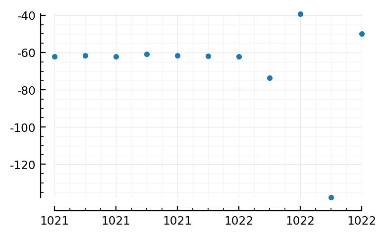
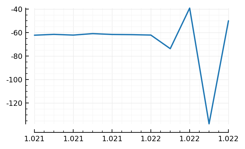
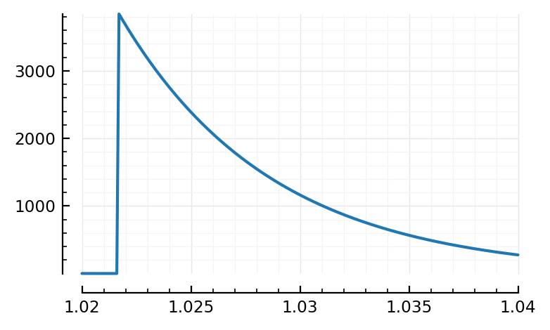
plotsig(s.timesteps, s.signals[696].v / mV, tlim=[1.021,1.022]);

plotsig(s.timesteps, s.signals[696].v / mV, tlim=[1.02,1.04])

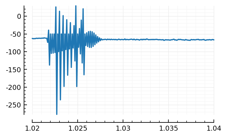
PyObject <AxesSubplot:>

plotsig(s.timesteps, s.signals[696].u / pA, tlim=[1.02,1.04]);

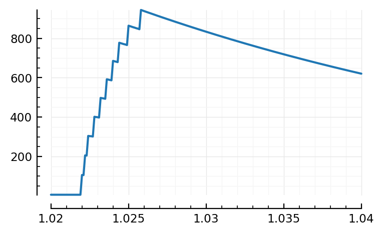
plotsig(s.timesteps, s.signals[696].g_inh / nS, tlim=[1.02,1.04]);

numspikes = length.(s.spike_times)

ComponentVector{Int64}(exc = [1, 3, 0, 0, 1, 0, 3, 1, 0, 1  …  1, 0, 0, 0, 1, 1, 2, 1, 0, 2], inh = [1, 1, 2, 2, 1, 3, 2, 3, 2, 1  …  1, 1, 2, 1, 0, 0, 4, 2, 3, 1])

findmax(numspikes)  # (val, index)

(58, 696)

s.spike_times[696] / ms

58-element Vector{Float64}:
  283.09999999998513
  283.2999999999851
  283.6999999999851
  284.099999999985
  284.499999999985
  284.8999999999849
  285.2999999999849
  285.69999999998487
  286.2999999999848
  951.6999999999115
  951.8999999999114
  952.0999999999115
  952.4999999999114
    ⋮
 1876.0999999998098
 1876.6999999998097
 2310.800000000452
 2311.0000000004525
 2311.4000000004535
 2311.800000000454
 2312.200000000455
 2312.600000000456
 2313.0000000004566
 2313.4000000004576
 2314.000000000459
 2315.0000000004607

Clusters, these always start a bit more than 10 ms (tx delay) after the input spikes of 812. (found by printing spiketimes of all 696’s inputs)

s.spike_times[812] / ms

6-element Vector{Float64}:
  272.39999999998633
  941.1999999999126
 1694.1999999998297
 1784.5999999998198
 1862.9999999998113
 2300.40000000043

labels(s.neuron_IDs)[812]

"inh[12]"

I wanna know if syn between these two is particularly strong.

[syn for syn in s.output_synapses[812] if s.postsyn_neuron[syn] == 696]

1-element Vector{Int64}:
 69244

s.syn_strengths[69244] / nS

3894.2034540205022

sort(s.syn_strengths[s.syns.inh_to_exc] / nS)

15923-element Vector{Float64}:
    1.9766044536578071
    2.188271086170034
    2.2988694124487004
    2.386741975213665
    2.5107083436583952
    2.5866747022907055
    2.6547608771121114
    2.749536896693771
    2.7665108323914187
    2.9194501336756873
    2.974603768194044
    3.1030473064492887
    3.1350052682906
    ⋮
 1968.049722427362
 1984.9063895892796
 1999.3965878497127
 2072.4237489509205
 2182.278608908274
 2273.2785123338335
 2467.500389769674
 3173.2421412651684
 3240.673205030154
 3894.2034540205022
 3899.103610867894
 5048.3299605142765

So our man has the second highest synaptic strength.

plt.hist(length.(values(s.input_neurons)));

More sanity check

p, s, spike_rates = sim_and_plot(
    duration = 3seconds,
    g_EE = 0,
    g_EI = 4,
    g_IE = 0,
    g_II = 0,
);

Running simulation: 100%|███████████████████████████████| Time: 0:00:04
Saving output at `C:\Users\tfiers\.phdcache\datamodel v2 (net)\sim\672f35a5c394ef4f.jld2` … done (0.7 s)

p, s, spike_rates = sim_and_plot(
    duration = 3seconds,
    g_EE = 1,
    g_EI = 0,
    g_IE = 0,
    g_II = 0,
);

Running simulation: 100%|███████████████████████████████| Time: 0:00:03
Saving output at `C:\Users\tfiers\.phdcache\datamodel v2 (net)\sim\254ca9b5e1177bf4.jld2` … done (0.7 s)

p, s, spike_rates = sim_and_plot(
    duration = 3seconds,
    g_EE = 0,
    g_EI = 0,
    g_IE = 0,
    g_II = 400,
);

Running simulation: 100%|███████████████████████████████| Time: 0:00:04
Saving output at `C:\Users\tfiers\.phdcache\datamodel v2 (net)\sim\2b7013ee6055458c.jld2` … done (0.5 s)

Params to do conntest with

plotsig(s.timesteps, s.signals[1].v)

PyObject <AxesSubplot:>

d = 8
p, s, spike_rates = sim_and_plot(
    duration = 30seconds,
    p_conn = 0.04,
    g_EE = 1   / d,
    g_EI = 18  / d,
    g_IE = 36  / d,
    g_II = 31  / d,
    ext_current = Normal(-0.5 * pA/√seconds, 5 * pA/√seconds),
    E_inh = -80 * mV,
);
# This is based on above, "pos mean input current" & roxin

Running simulation: 100%|███████████████████████████████| Time: 0:00:33
Saving output at `C:\Users\tfiers\.phdcache\datamodel v2 (net)\sim\56c7922ed33f58e2.jld2` … done (0.3 s)

Distributions same width if 3 or 30 seconds. good.

d = 6
p, s, spike_rates = sim_and_plot(
    duration = 3seconds,
    p_conn = 0.04,
    g_EE = 1   / d,
    g_EI = 18  / d,
    g_IE = 36  / d,
    g_II = 31  / d,
    ext_current = Normal(-0.5 * pA/√seconds, 5 * pA/√seconds),
    E_inh = -80 * mV,
);
# This is based on above, "pos mean input current" & roxin

Running simulation: 100%|███████████████████████████████| Time: 0:00:04
Saving output at `C:\Users\tfiers\.phdcache\datamodel v2 (net)\sim\35f3dc9269315d68.jld2` … done (0.2 s)

d = 6
p = get_params(
    duration = 10minutes,
    p_conn = 0.04,
    g_EE = 1   / d,
    g_EI = 18  / d,
    g_IE = 36  / d,
    g_II = 31  / d,
    ext_current = Normal(-0.5 * pA/√seconds, 5 * pA/√seconds),
    E_inh = -80 * mV,
    to_record = [1, 801],
);
s = cached(sim, [p.sim]);

Running simulation: 100%|███████████████████████████████| Time: 0:14:37
Saving output at `C:\Users\tfiers\.phdcache\datamodel v2 (net)\sim\d870417302bc9f1c.jld2` … done (1.6 s)

previous

2022-07-05 • Network conntest Roxin params

next

2022-05-13 • Network