2023-08-30__STA_examples¶

(Result of workflow speed (& ergonomy) tests: full Julia (no Python hybrid))

So, for all 10 Ns;
For 10 diff seeds; for both exc, inh, and unconn;
we conntest (maximum) 100 input spike trains.
(Each test is comprised of calculating 101 STAs: one real and the rest with shuffled ISIs).

From the prev nb (https://tfiers.github.io/phd/nb/2023-08-16__STA_conntest_pyjulia.html), we found we’d take a shorter window, so that ‘area over start’ measure (to determine if exc or inh) is correct.

But ok, it’s good to show that in thesis.
So, we repeat an example STA plot here.

for full N ofc.

include("lib/Nto1.jl")

using Revise … ✔ (0.3 s)
using Units, Nto1AdEx, ConnectionTests, ConnTestEval … 

[ Info: Precompiling Nto1AdEx [368485ca-63bc-4029-854f-349d2205662c]

✔ (1.5 s)
using StatsBase … ✔ (0.2 s)

N = 6500;

duration = 10minutes

@time sim = Nto1AdEx.sim(N, duration);

  2.994944 seconds (2.14 M allocations: 1.027 GiB, 2.34% gc time, 42.14% compilation time)

(1st run: 2.5 secs, 27% compilation time).

We want our input spiketrains sorted: the highest spikers first.
And split exc/inh, too.

include("lib/df.jl")

using DataFrames … ✔ (0.7 s)

exc_inputs = highest_firing(excitatory_inputs(sim))

tabulate(trains) = DataFrame(
    "# input spikes" => num_spikes.(trains),
    "spike rate (Hz)" => spikerate.(trains)
)
tabulate(exc_inputs)

5200×2 DataFrame

5190 rows omitted

Row	# input spikes	spike rate (Hz)
	Int64	Float64
1	58522	97.5
2	35312	58.9
3	24428	40.7
4	20653	34.4
5	18898	31.5
&vellip;	&vellip;	&vellip;
5196	194	0.323
5197	185	0.308
5198	175	0.292
5199	168	0.28
5200	123	0.205

inh_inputs = highest_firing(inhibitory_inputs(sim))

tabulate(inh_inputs)

1300×2 DataFrame

1290 rows omitted

Row	# input spikes	spike rate (Hz)
	Int64	Float64
1	21808	36.3
2	21054	35.1
3	16402	27.3
4	14905	24.8
5	14429	24
&vellip;	&vellip;	&vellip;
1296	234	0.39
1297	220	0.367
1298	218	0.363
1299	197	0.328
1300	140	0.233

( :) )

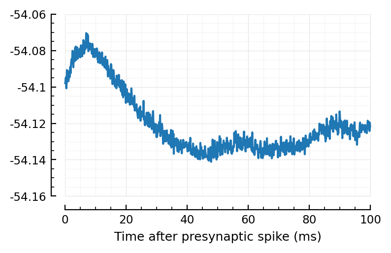
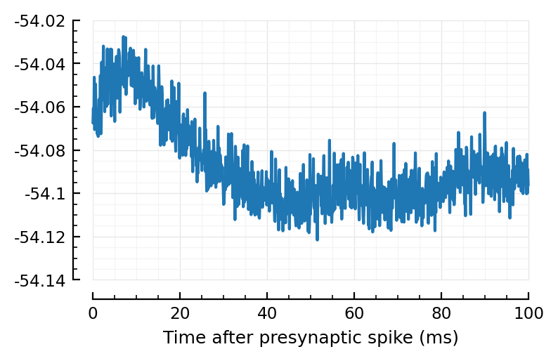
STA = calc_STA(sim.V, exc_inputs[1].times);

include("lib/plot.jl")

import PythonCall … ✔ (2 s)
import PythonPlot … ✔ (3.7 s)
using Sciplotlib … ✔ (0.5 s)
using PhDPlots … ✔

plotSTA(STA);

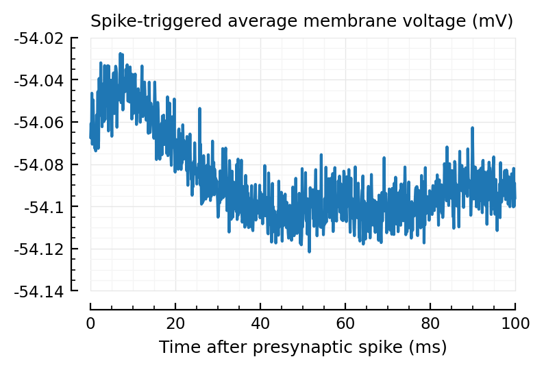
../_images/2023-08-30__STA_examples_17_0.png

To compare with predicted PSP height (0.04 mV):

(maximum(STA) - first(STA)) / mV

0.0399

(Woah, that’s close)

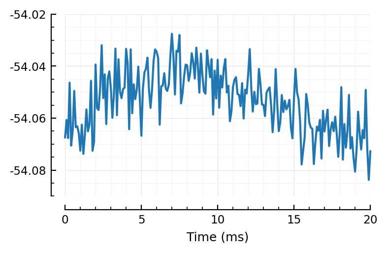
plotsig(STA/mV, [0,20], ms);

../_images/2023-08-30__STA_examples_21_0.png

plotSTA_(train, sim=sim; kw...) = begin
    nspikes = num_spikes(train)
    EI = train ∈ exc_inputs ? "exc" : "inh"
    label = "$nspikes spikes, $EI"
    plotSTA(calc_STA(sim.V, train.times); label, kw...)
end
    
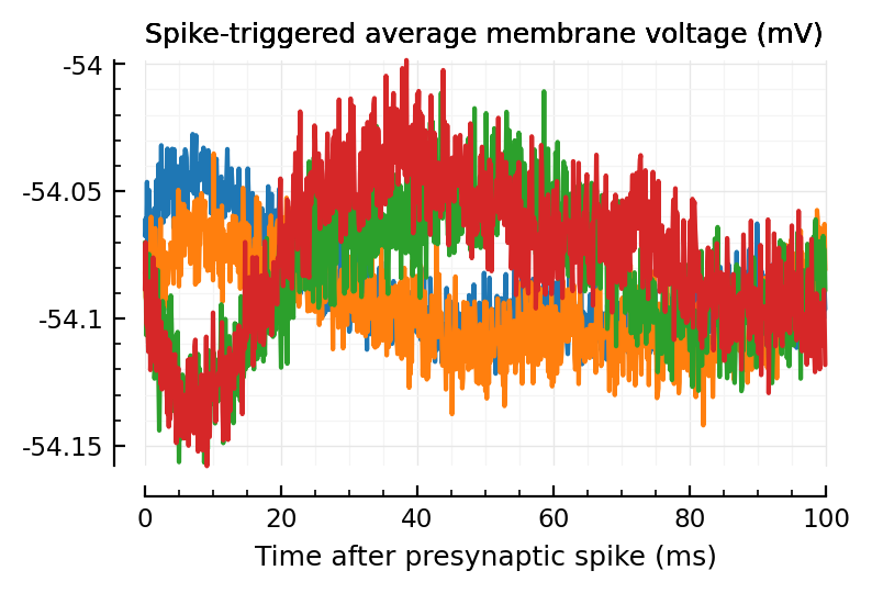
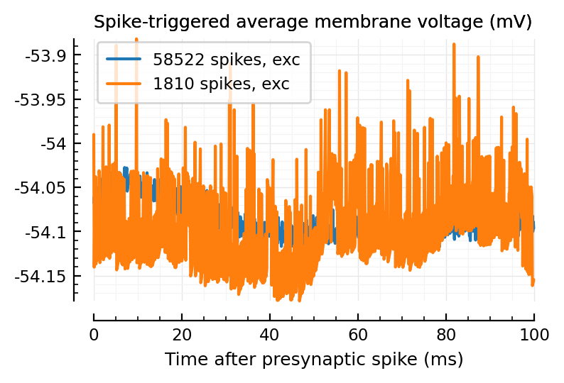
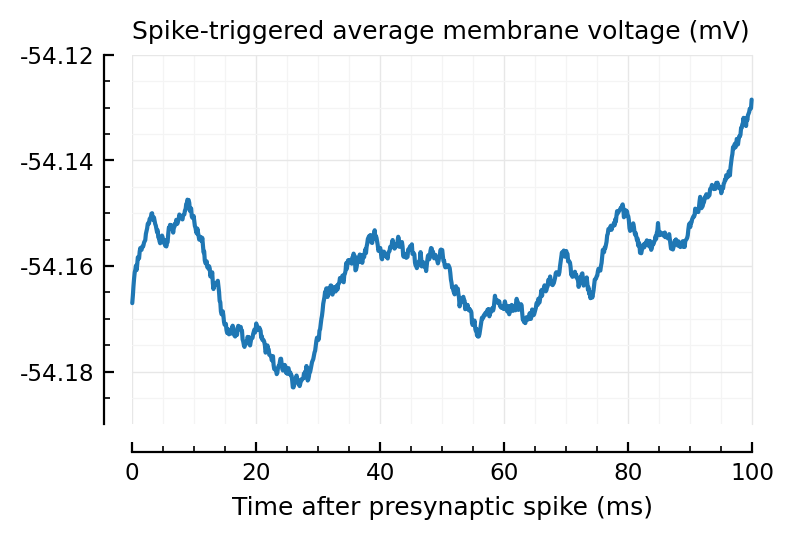
plotSTA_(exc_inputs[1]);
plotSTA_(exc_inputs[2]);
plotSTA_(inh_inputs[1]);
plotSTA_(inh_inputs[2]);

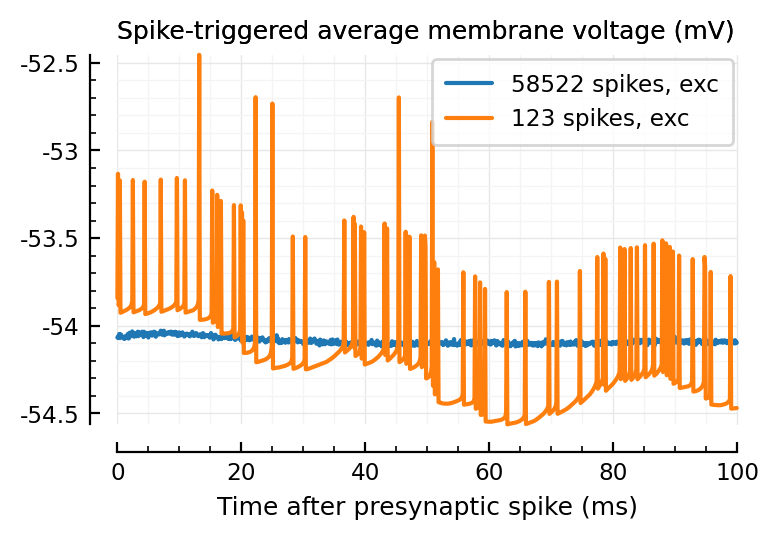
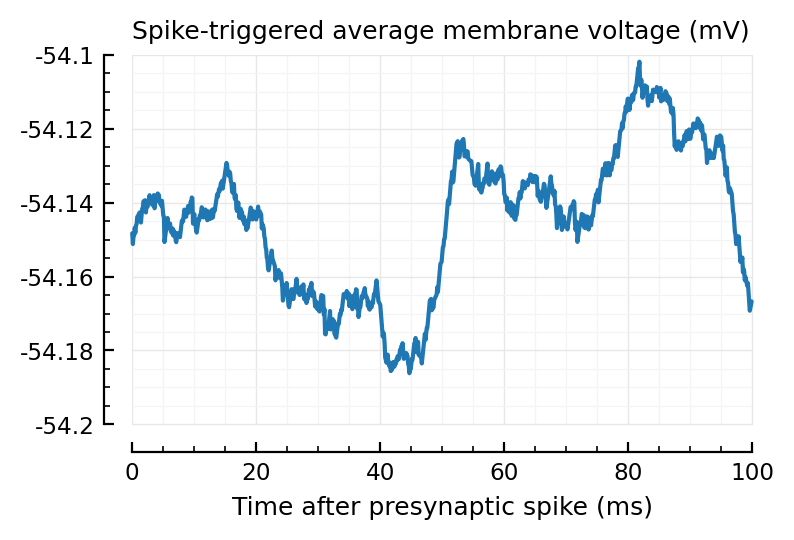
../_images/2023-08-30__STA_examples_22_0.png

plotSTA_(exc_inputs[1]);
plotSTA_(exc_inputs[end]);
plt.legend();

../_images/2023-08-30__STA_examples_23_0.png

mid = length(exc_inputs) ÷ 2

plotSTA_(exc_inputs[1]);
plotSTA_(exc_inputs[mid]);
plt.legend();

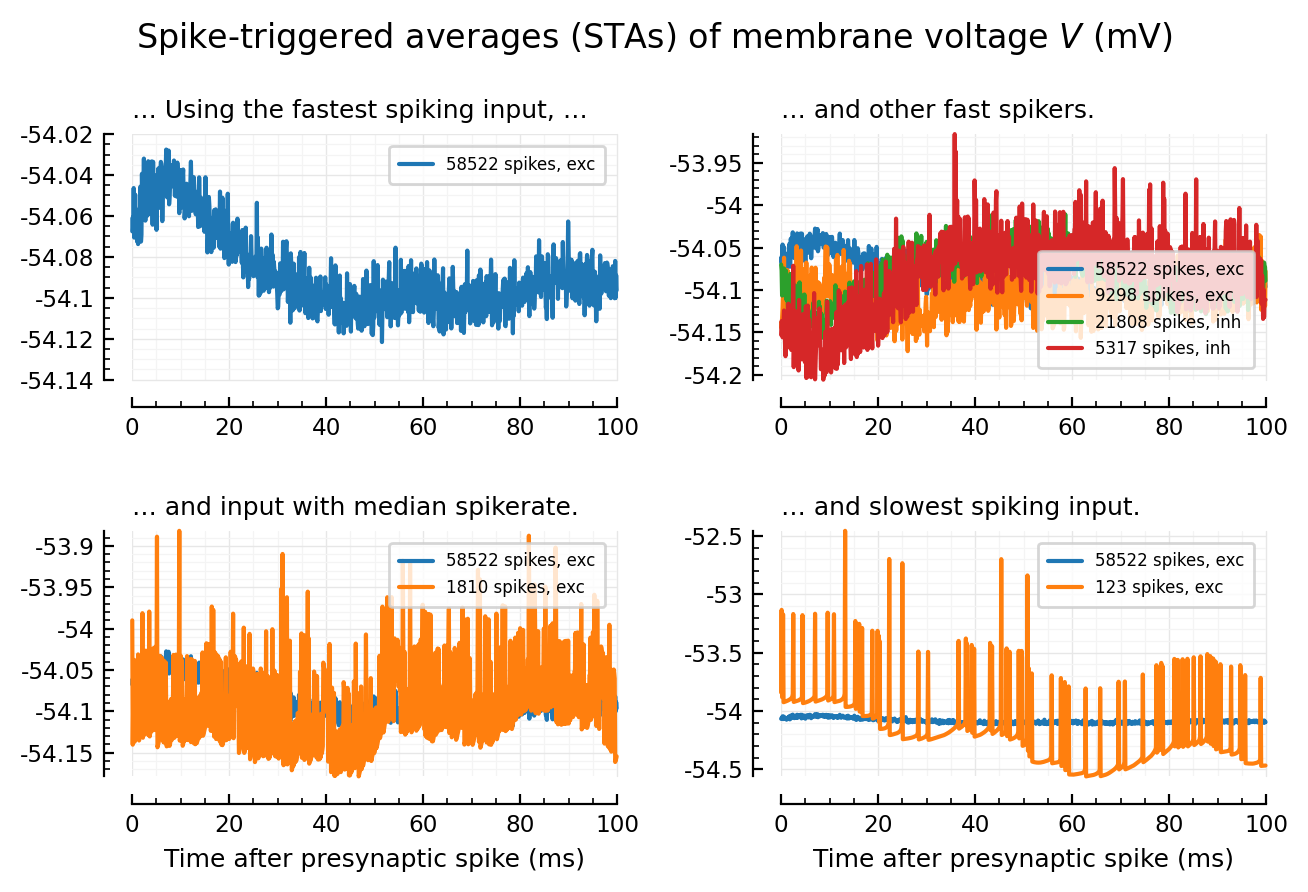
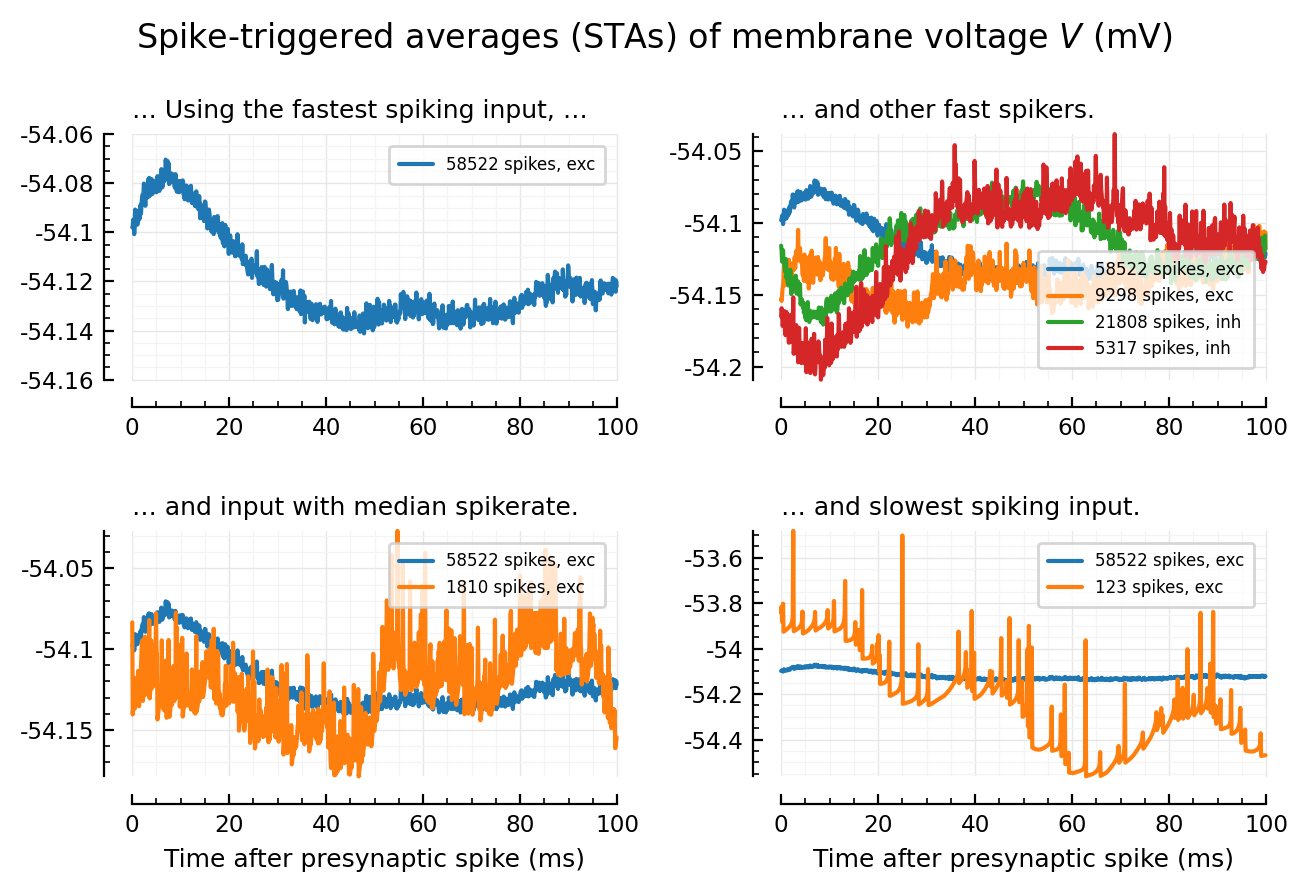
../_images/2023-08-30__STA_examples_24_0.png

Four-panel plot¶

fig, axs = plt.subplots(nrows=2, ncols=2, figsize=(pw*0.8, mtw))
plotSTA_2(args...; hylabel=nothing, kw...) = plotSTA_(args...; hylabel, kw...)

addlegend(ax; kw...) = legend(ax, fontsize=6, borderaxespad=0.7; kw...)

plotSTA_2(exc_inputs[1], ax=axs[0,0], hylabel="… Using the fastest spiking input, …", xlabel=nothing);
addlegend(axs[0,0])

plotSTA_2(exc_inputs[1], ax=axs[0,1], hylabel="… and other fast spikers.", xlabel=nothing);
plotSTA_2(exc_inputs[100], ax=axs[0,1], xlabel=nothing)
plotSTA_2(inh_inputs[1], ax=axs[0,1], xlabel=nothing)
plotSTA_2(inh_inputs[100], ax=axs[0,1], xlabel=nothing)
addlegend(axs[0,1], loc="lower right")


plotSTA_2(exc_inputs[1], ax=axs[1,1], hylabel="… and slowest spiking input.");
plotSTA_2(exc_inputs[end], ax=axs[1,1]);
addlegend(axs[1,1])

plotSTA_2(exc_inputs[1], ax=axs[1,0], hylabel="… and input with median spikerate.");
plotSTA_2(exc_inputs[mid], ax=axs[1,0]);
addlegend(axs[1,0], loc="upper right")

plt.suptitle(L"Spike-triggered averages (STAs) of membrane voltage $V$ (mV)")

plt.tight_layout(h_pad=2);

# savefig_phd("example_STAs")

../_images/2023-08-30__STA_examples_26_0.png

fig, axs = plt.subplots(nrows=2, ncols=2, figsize=(pw*0.8, mtw))
plotSTA_2(args...; hylabel=nothing, kw...) = plotSTA_(args...; hylabel, kw...)

addlegend(ax; kw...) = legend(ax, fontsize=6, borderaxespad=0.7; kw...)

plotSTA_2(exc_inputs[1], ax=axs[0,0], hylabel="… Using the fastest spiking input, …", xlabel=nothing);
addlegend(axs[0,0])

plotSTA_2(exc_inputs[1], ax=axs[0,1], hylabel="… and other fast spikers.", xlabel=nothing);
plotSTA_2(exc_inputs[100], ax=axs[0,1], xlabel=nothing)
plotSTA_2(inh_inputs[1], ax=axs[0,1], xlabel=nothing)
plotSTA_2(inh_inputs[100], ax=axs[0,1], xlabel=nothing)
addlegend(axs[0,1], loc="lower right")


plotSTA_2(exc_inputs[1], ax=axs[1,1], hylabel="… and slowest spiking input.");
plotSTA_2(exc_inputs[end], ax=axs[1,1]);
addlegend(axs[1,1])

plotSTA_2(exc_inputs[1], ax=axs[1,0], hylabel="… and input with median spikerate.");
plotSTA_2(exc_inputs[mid], ax=axs[1,0]);
addlegend(axs[1,0], loc="upper right")

plt.suptitle(L"Spike-triggered averages (STAs) of membrane voltage $V$ (mV)")

plt.tight_layout(h_pad=2);

# savefig_phd("example_STAs")

Saved at `../thesis/figs/example_STAs.pdf`

../_images/2023-08-30__STA_examples_27_1.png

(For colour in figure caption text):

cs = darken.(Sciplotlib.mplcolors, 0.87)

../_images/2023-08-30__STA_examples_29_0.svg

toRGBAtuple.(cs)[1:6]

6-element Vector{NTuple{4, FixedPointNumbers.N0f8}}:
 (0.106N0f8, 0.408N0f8, 0.616N0f8, 1.0N0f8)
 (0.871N0f8, 0.431N0f8, 0.047N0f8, 1.0N0f8)
 (0.149N0f8, 0.545N0f8, 0.149N0f8, 1.0N0f8)
 (0.729N0f8, 0.133N0f8, 0.137N0f8, 1.0N0f8)
 (0.506N0f8, 0.353N0f8, 0.643N0f8, 1.0N0f8)
 (0.478N0f8, 0.294N0f8, 0.255N0f8, 1.0N0f8)

Ceil spikes¶

sim_ceil = deepcopy(sim)
ceil_spikes!(sim_ceil.V, sim_ceil.spiketimes);

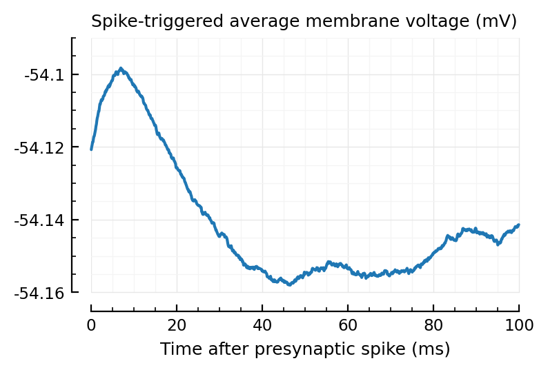
plotSTA_2(exc_inputs[1]);

../_images/2023-08-30__STA_examples_33_0.png

plotSTA_2(exc_inputs[1], sim_ceil);

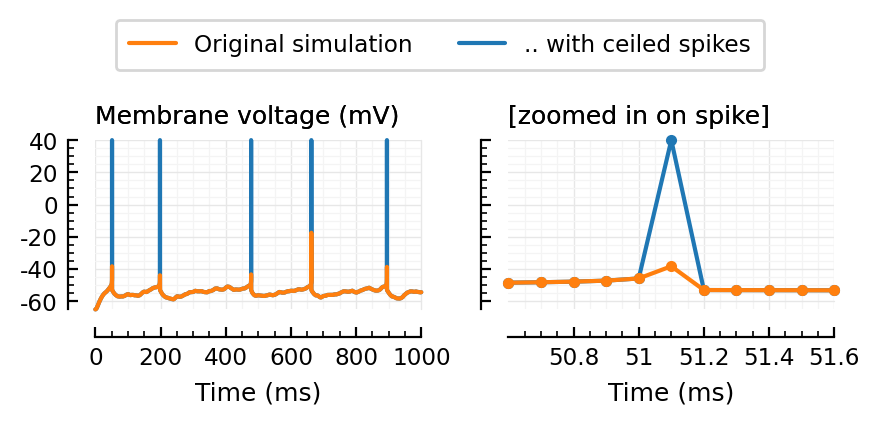
../_images/2023-08-30__STA_examples_34_0.png

Wow much worse, with ceiled spikes.

So, obviously, let’s try and trim the spikes.
Also, what’s voltage histogram ey.

hist(sim_ceil.V / mV);

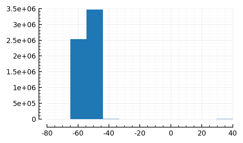
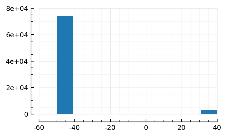
../_images/2023-08-30__STA_examples_37_0.png

V = sim_ceil.V
hist(V[V .≥ -50mV] / mV);

../_images/2023-08-30__STA_examples_38_0.png

Can we do automatic selection? percentiles let’s see. Or outlier detection, or sth.

using Statistics

ps = [0, 0.01, 0.5, 0.9, 0.99, 0.999, 1]  # i.e. 0, 1, 50, 90, 99, 99.1, 100-percentiles.
qs = quantile(V, ps) / mV
DataFrame("Proportion"=>ps, "Value (mV)"=>round.(qs, digits=1))

7×2 DataFrame

Row	Proportion	Value (mV)
	Float64	Float64
1	0.0	-65.0
2	0.01	-58.1
3	0.5	-54.0
4	0.9	-51.6
5	0.99	-49.8
6	0.999	-46.8
7	1.0	40.0

V_clip = copy(sim_ceil.V)
V_clip[V_clip .≥ -50mV] .= -50mV;

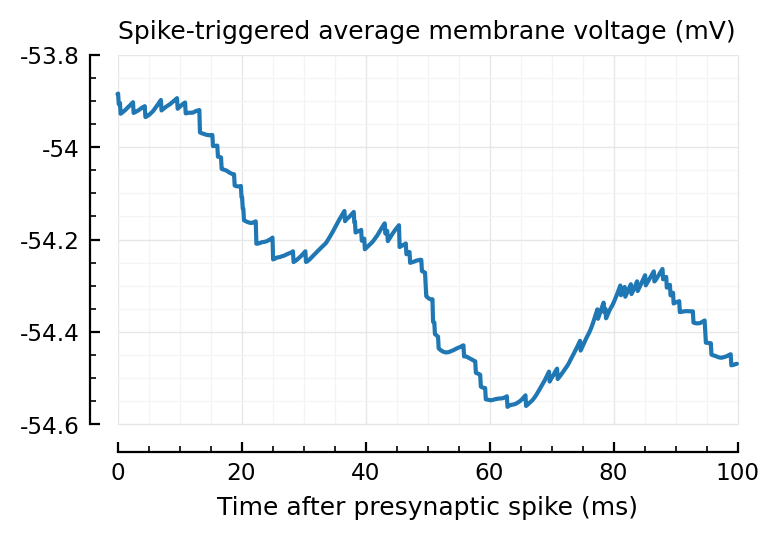
plotSTA(calc_STA(V_clip, exc_inputs[1].times));

../_images/2023-08-30__STA_examples_43_0.png

Holy damn :OOOO
This is so clean :OOOO.

plotSTA(calc_STA(V_clip, exc_inputs[100].times));

../_images/2023-08-30__STA_examples_45_0.png

plotSTA(calc_STA(V_clip, exc_inputs[mid].times));

../_images/2023-08-30__STA_examples_46_0.png

plotSTA(calc_STA(V_clip, exc_inputs[end].times));

../_images/2023-08-30__STA_examples_47_0.png

Ok no real help for the lower spikers heh.

Sig itself¶

function ceilplot(; tlim, marker=nothing, ax, kw...)
    plotsig(sim_ceil.V / mV, tlim, ms, label=".. with ceiled spikes"; ax, marker, kw...);
    plotsig(sim.V / mV, tlim, ms, label="Original simulation"; ax, marker, kw...);
    # legend(ax, reorder=[1=>2]);
end

fig, axs = plt.subplots(ncols=2, figsize=(mtw, 0.4*mtw), sharey=true)
ceilplot(tlim = [0, 1000], ax=axs[0], hylabel="Membrane voltage (mV)");
ceilplot(tlim = [50.6, 51.6], marker=".", ax=axs[1], hylabel="[zoomed in on spike]");
l = axs[0].get_lines()
# rm_ticks_and_spine(axs[1], "left")
plt.figlegend(handles=[l[1], l[0]], ncols=2, loc="lower center", bbox_to_anchor=(0.5, 1))
plt.tight_layout();

../_images/2023-08-30__STA_examples_50_0.png

‘What would V would be w/o thresholding’¶

@time sim_r = Nto1AdEx.sim(N, duration, record_all=true);

  2.686393 seconds (6.03 M allocations: 1.383 GiB, 25.27% gc time)

We need to calc V. Which is Vprev + Δt * ΔV

t = sim_r.spiketimes[1]
t / ms

51.200000000000436

(; Δt, Eₑ, Eᵢ, Δₜ, Vₜ, gₗ, Eₗ, C) = Nto1AdEx

i = round(Int, t/Δt)  # The spiketime `t` is one sample after where we want, but this i is correct

n = sim_r.recording[i];

(; V, gₑ, gᵢ, w) = n
V / mV

-38.24759825475466

n.DₜV

75.60870254277917

DₜV

966640.2938251279

Iₛ = gₑ*(V - Eₑ) + gᵢ*(V - Eᵢ)
DₜV  = (-gₗ*(V - Eₗ) + gₗ*Δₜ*exp((V-Vₜ)/Δₜ) - Iₛ - w) / C

V_new = V + Δt * DₜV
V_new / mV

96625.78178425804

Heh.

Voltage-to-Wiring Sim

2023-08-30__STA_examples

Contents

2023-08-30__STA_examples¶

Four-panel plot¶

Ceil spikes¶

Sig itself¶

‘What would V would be w/o thresholding’¶