2020-10-23 • Delete signal around spikes before STA
Contents
2020-10-23 • Delete signal around spikes before STA
This notebook is similar to /notebooks/2020-07-29__STA, /notebooks/2020-09-10__STA_for_different_PSP_shapes, and /notebooks/2020-09-18__Clip_spikes_before_STA.
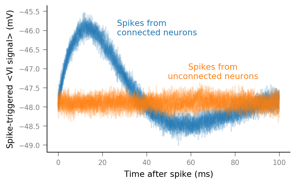
We still wonder whether the bump in the STA is due to averaging post synaptic potentials (PSPs), or postsynaptic spikes.
We clipped the signal, but this still kept the ramp-up of the membrane potential right before a spike. It might be this ramp-up that caused the bump (instead of PSPs).
Here we try to get rid of that ramp-up by deleting the VI signal around each spike (replacing it with NaN [“not a number”]).
We then repeat the STA window procedure to see if the bump is still there, or not.
Nothing new here
All sections nested under this are the same as in the three previous notebooks.
Imports & reproducibility info
from voltage_to_wiring_sim.notebook_init import *
Preloading:
 - numpy … (0.44 s)
 - matplotlib.pyplot … (0.57 s)
 - numba … (0.71 s)
 - sympy … (0.71 s)
 - unyt … (1.07 s)

Imported `np`, `mpl`, `plt
Imported package `voltage_to_wiring_sim` as `v`
Imported `*` from `v.util` and from `v.units`
Setup autoreload

Reproducibility info. This notebook was last run on/with:

Mon Oct 26 2020 10:47:13 Romance Standard Time

CPython 3.8.3
IPython 7.18.1

compiler   : MSC v.1916 64 bit (AMD64)
system     : Windows
release    : 10
machine    : AMD64
processor  : Intel64 Family 6 Model 142 Stepping 12, GenuineIntel
CPU cores  : 8
interpreter: 64bit
host name  : yoga
Git hash   : 531bc468b35e14e2c5748ac51a380d0f70575615
Git repo   : git@github.com:tfiers/voltage-to-wiring-sim.git
Git branch : main
Time grid
tg = v.TimeGrid(T=10 * minute, dt=0.1 * ms)
TimeGrid(T=Quantity(10 min, stored in s, float64), dt=Quantity(0.1 ms, stored in s, float64), N=unyt_quantity(6000000, '(dimensionless)'), t=Array([0 1.667E-06 3.333E-06 ... 10 10 10] min, stored in s, float64))
Spike trains
‘Network’ definition.
N_in = 30
p_connected = 0.5

N_connected = round(N_in * p_connected)
N_unconnected = N_in - N_connected
15
Have all incoming neurons spike with the same mean frequency, for now.
f_spike = 20 * Hz
Quantity(20 Hz, stored in Hz, float64)
gen_st = v.generate_Poisson_spike_train

fix_rng_seed()
%%time
spike_trains_connected = [gen_st(tg, f_spike) for _ in range(N_connected)]
spike_trains_unconnected = [gen_st(tg, f_spike) for _ in range(N_unconnected)]
Wall time: 1.48 s
all_spike_trains = spike_trains_connected + spike_trains_unconnected;
Time slice
Inspect a time excerpt..
time_slice = 1 * minute + [0, 1] * second

slice_indices = np.round(time_slice / tg.dt).astype(int)
i_slice = slice(*slice_indices)
t_slice = tg.t[i_slice].in_units(second);
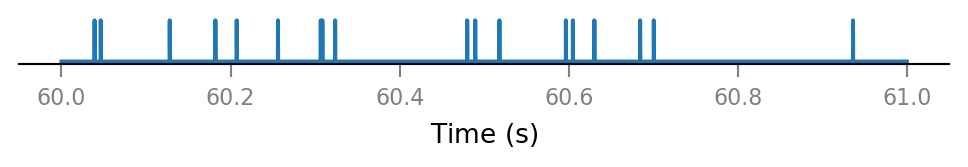
..of one presynaptic neuron:
v.spike_train.plot(t_slice, all_spike_trains[0][i_slice]);
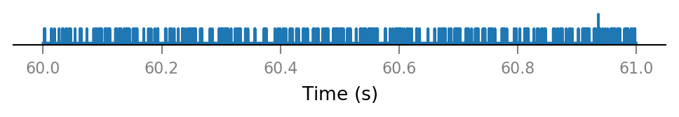
All connected presynaptic neurons:
all_incoming_spikes = sum(spike_trains_connected)

v.spike_train.plot(t_slice, all_incoming_spikes[i_slice]);
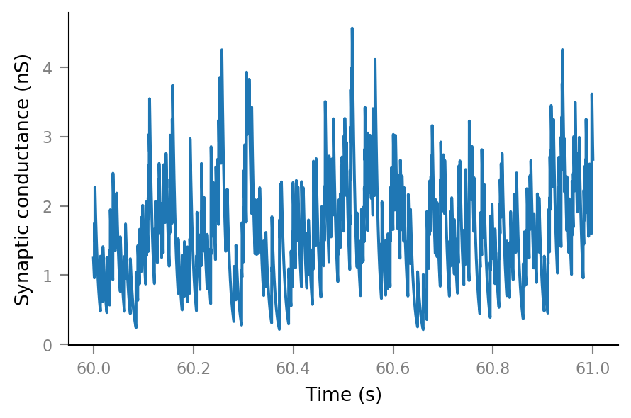
Synaptic conductance
Δg_syn = 0.8 * nS
τ_syn = 7 * ms;
g_syn = v.calc_synaptic_conductance(tg, all_incoming_spikes, Δg_syn, τ_syn)

plt.plot(t_slice, g_syn[i_slice]);
Membrane voltage
params = v.params.cortical_RS
print(params)
IzhikevichParams
----------------
C = 100 pF
k = 0.7 nS/mV
v_r = -60 mV
v_t = -40 mV
v_peak = 35 mV
a = 0.03 1/ms
b = -2 nS
c = -50 mV
d = 100 pA
v_syn = 0 mV
%%time
sim = v.simulate_izh_neuron(tg, params, g_syn)
Wall time: 345 ms
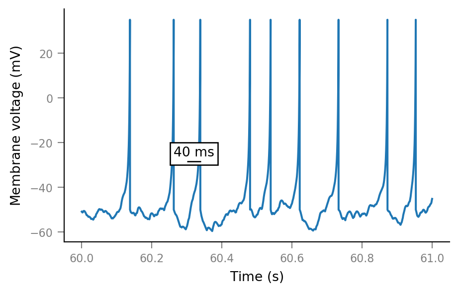
fig, ax = plt.subplots()
ax.plot(t_slice, sim.V_m[i_slice])
add_scalebar(ax, 40 * ms, x=60.32*second, y=-25*mV, frame=True);
Noise
SNR = 10
spike_height = params.v_peak - params.v_r
σ_noise = spike_height / SNR
noise = np.random.randn(tg.N) * σ_noise
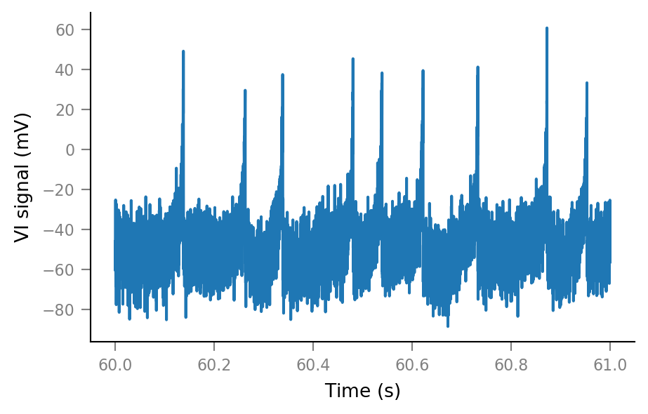
Vm_noisy = (sim.V_m + noise).in_units(mV)
Vm_noisy.name = "VI signal"
plt.plot(t_slice, Vm_noisy[i_slice]);
Find spike times
(Later we’ll save spike times at simulation time. For now we detect them post hoc).
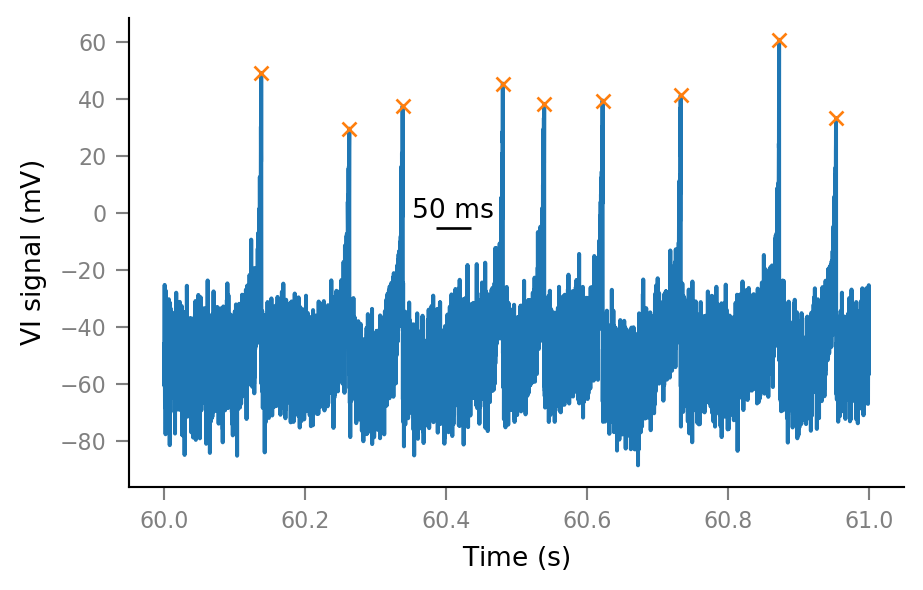
from scipy.signal import find_peaks
spikes_ix, _ = find_peaks(Vm_noisy, height=(10 * mV).item(), distance=4 * ms / tg.dt)
height argument is minimum peak height.
Peaks are removed, lowest first, until the “distance between peaks” argument is satisfied
i_start, i_end = slice_indices
spike_ix_slice = spikes_ix[(spikes_ix > i_start) & (spikes_ix < i_end)]

fig, ax = plt.subplots()
ax.plot(t_slice, Vm_noisy[i_slice])
ax.plot(tg.t[spike_ix_slice], Vm_noisy[spike_ix_slice], "x", ms=5)
add_scalebar(ax, 50 * ms, x=60.41 * second, y=0 * mV);
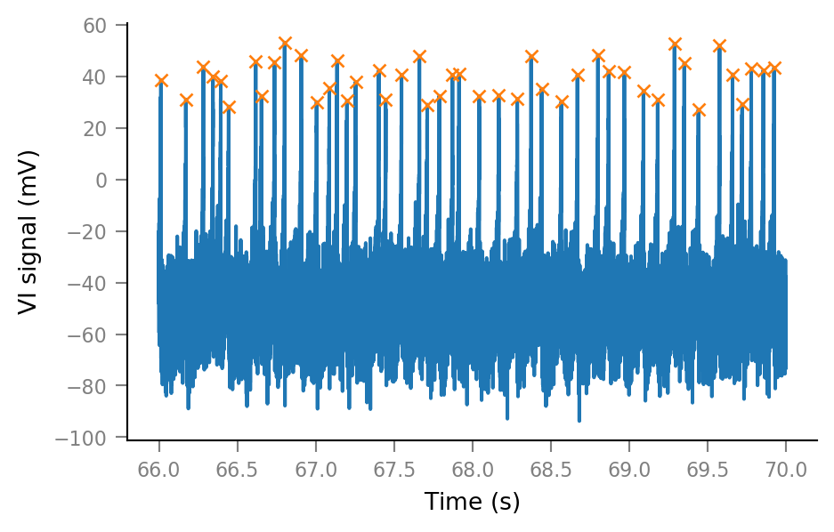
New extended time slice:
time_slice2 = 66 * second + [0, 4] * second
# time_slice2 = 66.6 * second + [0, 100] * ms

slice_indices2 = np.round(time_slice2 / tg.dt).astype(int)
i_slice2 = slice(*slice_indices2)
t_slice2 = tg.t[i_slice2].in_units(second);
i_start2, i_end2 = slice_indices2
spike_ix_slice2 = spikes_ix[(spikes_ix > i_start2) & (spikes_ix < i_end2)]

plt.plot(t_slice2, Vm_noisy[i_slice2])
plt.plot(tg.t[spike_ix_slice2], Vm_noisy[spike_ix_slice2], "x", ms=5);
Delete signal around spikes
deletion_frame = [-60 * ms, 20 * ms]; # relative to spike time
deletion_frame_ix = np.array(deletion_frame) / tg.dt.data;

Vm_noisy_redacted = Vm_noisy.copy()

for spike_ix in spikes_ix:
    deletion_ix_slice = slice(*(spike_ix + deletion_frame_ix).astype(int))
    Vm_noisy_redacted[deletion_ix_slice] = np.nan
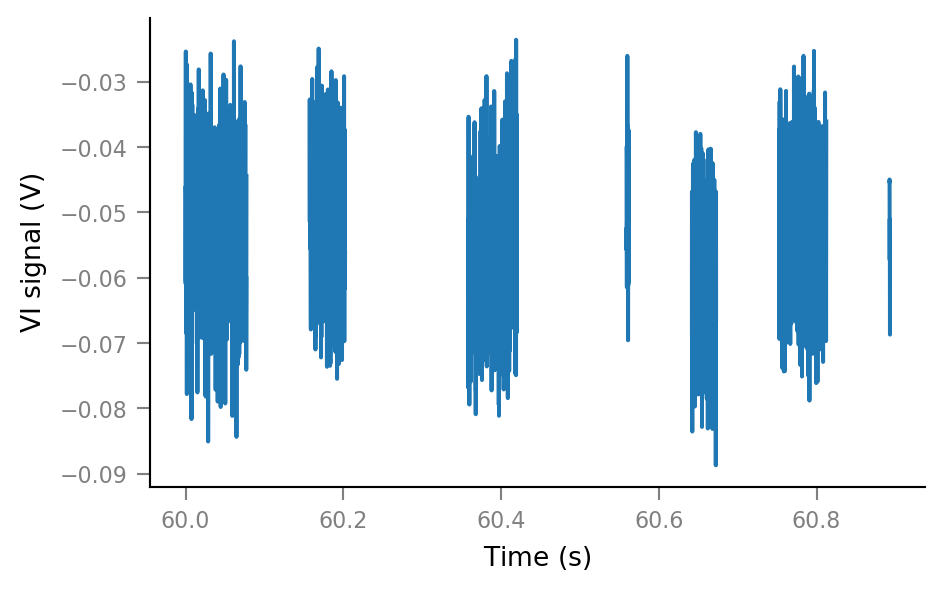
plt.plot(t_slice, Vm_noisy_redacted[i_slice]);
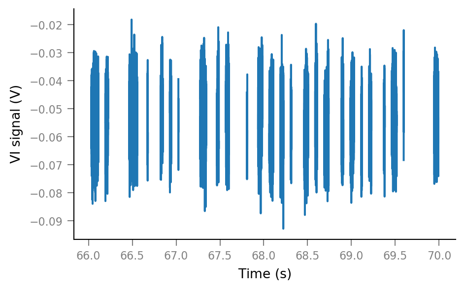
plt.plot(t_slice2, Vm_noisy_redacted[i_slice2]);
Spike-triggered windows
def get_spike_indices(spike_train):
    # `nonzero` returns a tuple (one element for each array dimension).
    (spike_indices,) = np.nonzero(spike_train)
    return spike_indices
Extract windows from the VI signal.
window_length = 100 * ms

window_tg = v.TimeGrid(window_length, tg.dt)
window_tg.t.name = "Time after spike"


# Performance
Vm_noisy_redacted_arr = np.asarray(Vm_noisy_redacted)
window_tg_N = window_tg.N
tg_N = tg.N

import numba

@numba.njit
def _make_windows(spike_indices):
    windows = []
    for ix in spike_indices:
        ix_end = ix + window_tg_N
        if ix_end < tg_N:
            windows.append(Vm_noisy_redacted_arr[ix:ix_end])

    return windows

def make_windows(spike_indices):
    windows = np.stack(_make_windows(spike_indices))
    return Array(windows, V, name=Vm_noisy_redacted.name).in_units(mV)
spike_train__example = all_spike_trains[0]
spike_indices__example = get_spike_indices(spike_train__example)
windows__example = make_windows(spike_indices__example)
windows__example.shape
(12019, 1000)
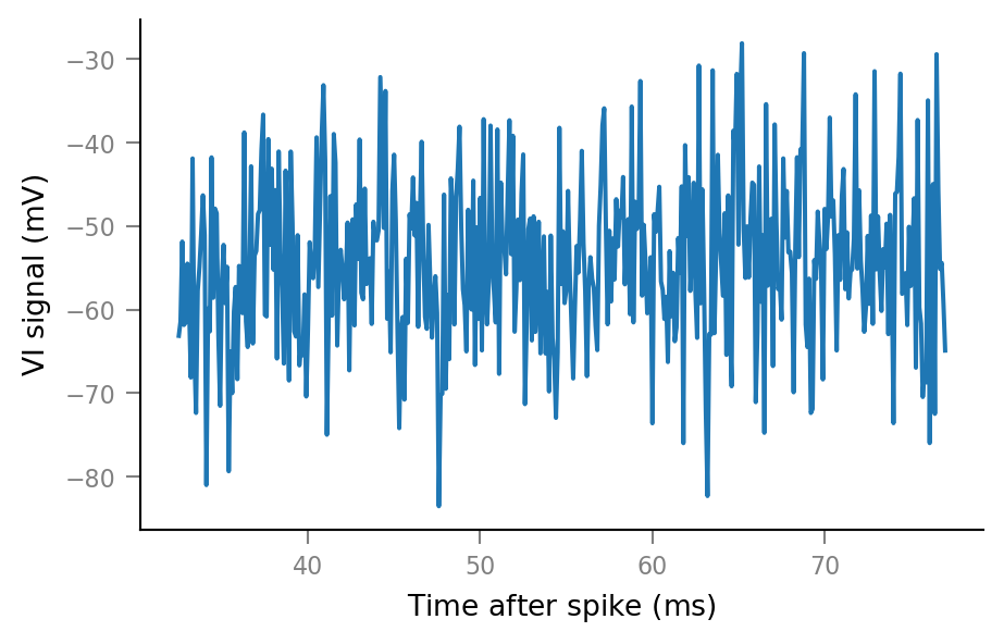
An example spike-triggered window:
plt.plot(window_tg.t, windows__example[0, :]);
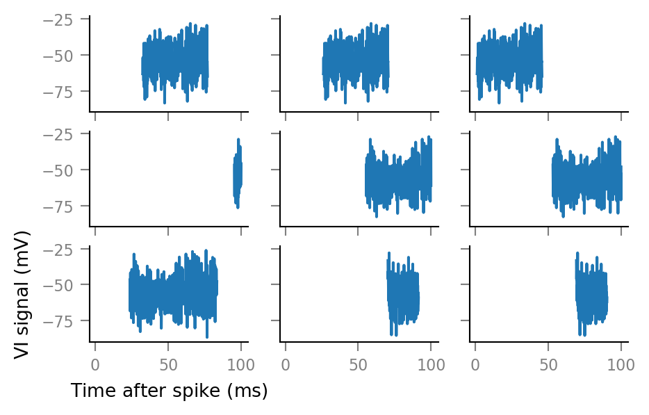
And some more:
fig, axes = plt.subplots(nrows=3, ncols=3, sharex=True, sharey=True)

for row, row_axes in enumerate(axes):
    for col, ax in enumerate(row_axes):
        i = 3 * row + col
        ax.plot(window_tg.t, windows__example[i, :])
        if not (row == 2 and col == 0):
            ax.set(xlabel=None, ylabel=None)
Average windows
Note that we use nanmean, which ignores deleted values (NaN) when taking the mean (instead of making the whole mean result NaN).
def STA(spike_train):
spike_indices = get_spike_indices(spike_train)
windows = make_windows(spike_indices)
STA = np.nanmean(windows, axis=0)
return Array(STA, V, name="Spike-triggered <VI signal>").in_units(mV)
def plot_STA(spike_train, ax=None, **kwargs):
if ax is None:
fig, ax = plt.subplots()
ax.plot(window_tg.t, STA(spike_train), **kwargs)
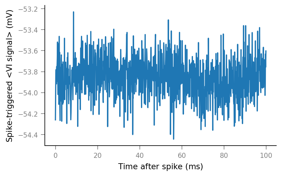
plot_STA(spike_trains_connected[0])
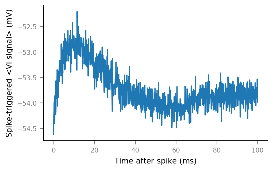
plot_STA(spike_trains_unconnected[0])
Plot STAs of all spike trains
%%time

fig, ax = plt.subplots()

for spike_train in spike_trains_connected:
    plot_STA(spike_train, ax, alpha=0.2, color='C0')

for spike_train in spike_trains_unconnected:
    plot_STA(spike_train, ax, alpha=0.2, color='C1')

plt.close()
Wall time: 16.9 s
# Clear existing texts, for iterative positioning.
for _ in range(len(ax.texts)):
    ax.texts.pop()

ax.annotate(
    "Spikes from\nconnected neurons",
    xy=(26.55 * ms, 0.8),
    xycoords=("data", "axes fraction"),
    color="C0",
    ha="left",
)

ax.annotate(
    "Spikes from\nunconnected neurons",
    xy=(70 * ms, 0.5),
    xycoords=("data", "axes fraction"),
    color="C1",
    ha="center",
)

fig
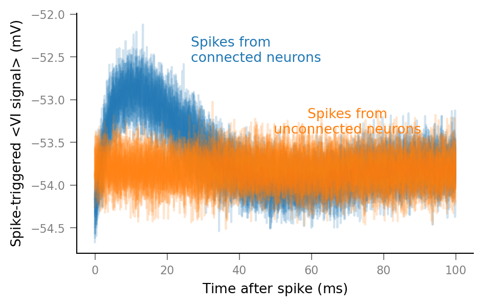
This was the first STAs plot, without any deletions: